Grok Critiques SD

Just for fun, I asked Grok for a list of critiques, and it came up with a pretty good one. [I’ve added a few notes and references in brackets.]

System Dynamics (SD) modeling, while powerful for analyzing complex systems, faces several critiques:

  1. Oversimplification: SD models often simplify complex systems, potentially missing critical details or interactions, leading to inaccurate predictions or insights. [One example of this is the Axtell critique of aggregation, which is a bit of a strawdog.]
  2. Subjectivity in Model Design: Model boundaries, assumptions, and relationships are defined by modelers, which can introduce bias or limit the model’s applicability. [See Dana Meadows’ Unavoidable A Priori.]
  3. Data Dependency: SD relies heavily on accurate data for calibration and validation. Poor-quality or incomplete data can undermine model reliability. [This is ironic, because SD historically did not rely heavily on formal data, and that is the usual critique. But SD provides excellent ways to improve reliability by combining data with sensible structure.]
  4. Difficulty in Validation: Validating SD models is challenging, especially for long-term predictions, as real-world systems evolve unpredictably, and historical data may not suffice. [What method doesn’t have this problem, other than trivial ones that are easy to reject?]
  5. Computational Complexity: Large SD models can be computationally intensive, making them difficult to scale or analyze in real-time scenarios. [Yep.]
  6. Limited Predictive Power: SD is better suited for understanding system behavior than precise forecasting, as it struggles with chaotic or highly stochastic systems. [Nope.]
  7. Misinterpretation Risk: Non-experts may misinterpret model outputs, assuming deterministic results rather than recognizing them as scenarios or trends. [True, but hardly unique to SD. See Communicating uncertainty and policy sensitivity]
  8. Neglect of Discrete Events: SD focuses on continuous processes, which may inadequately capture discrete events or abrupt changes in systems. [Common, but not a requirement, even in the early days of SD.]
  9. Resistance to Interdisciplinary Integration: Some critics argue SD struggles to integrate with other modeling approaches (e.g., agent-based modeling), limiting its flexibility. [It might be a struggle, but I don’t think deliberate resistance is the issue.]
  10. Overemphasis on Feedback Loops: While feedback loops are central to SD, overfocusing on them can downplay external drivers or one-off events impacting the system. [Consider George Richardson’s endogenous point of view.]

These critiques highlight the need for careful model design, validation, and clear communication of limitations when using SD. Would you like me to dive deeper into any specific critique?
Conveyor Causality is Wrong

Both Stella and Vensim draw conveyors incorrectly, in different ways.

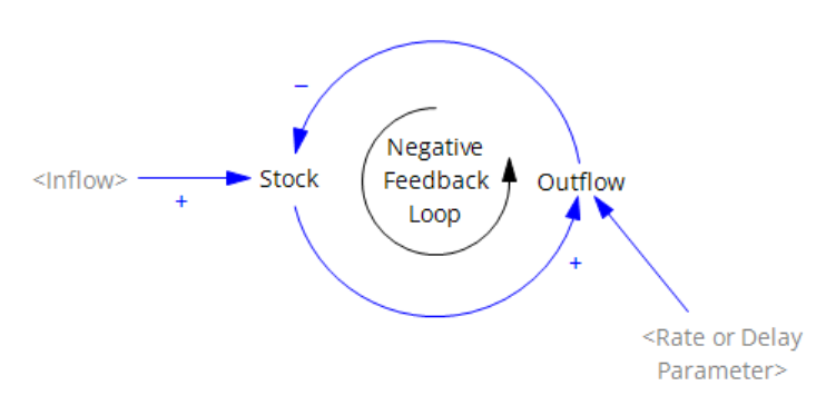
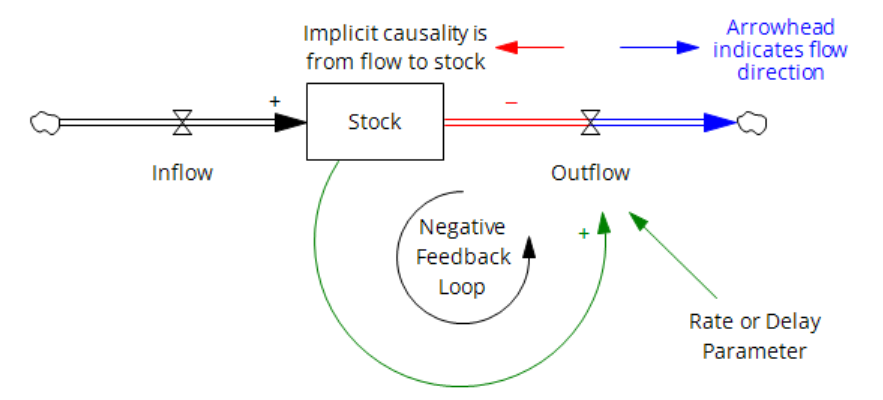
In part, the challenges arise from the standard SD convention for stock-flow diagramming. Consider the stock-flow structure above and its CLD equivalent below.

The CLD version has its own problems, but the stock-flow version is potentially baffling to novices because the arrowhead convention for flow pipes differs from an information arrow in its representation of causality. The arrowhead indicates the direction of material flow, which is the opposite of the direction of causality or information. In Stella, there may be a “shadow” arrowhead in the negative-flow direction, but this doesn’t really help – the concept of flow direction (bidirectional vs. unidirectional) is still confounded with causality (always flow->stock).

When the stock is a conveyor, the problems deepen.

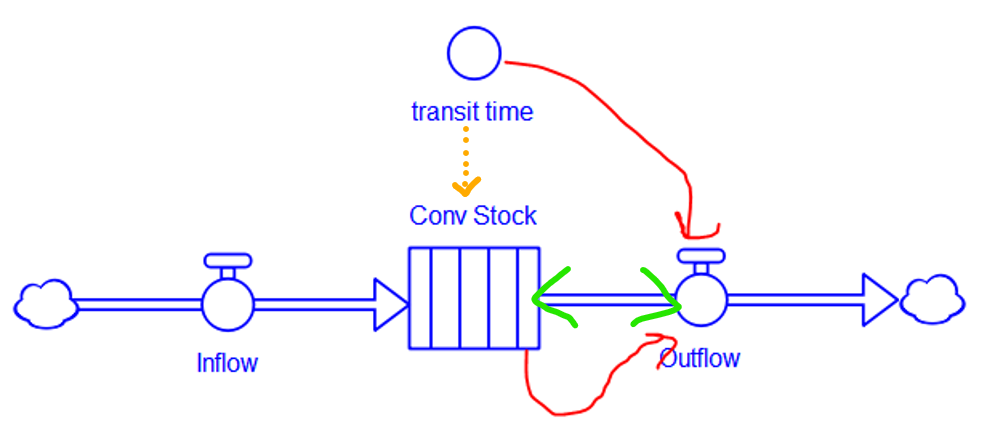
In Stella, the conveyor has a distinct icon, which is good. It indicates that the stock is divided into internal compartments (which are essentially slats of TIME STEP aka DT duration, rendering the object higher-order than a normal stock). However, the transit time is a property setting in the stock dialog, implying the orange arrow, which can’t properly be drawn because stocks don’t normally have dynamic information arrow inputs, and transit time could potentially change during the simulation. The segment of flow pipe between the stock and outflow is now further overloaded, because it represents both the “expiration” of stock contents due to exceedance of transit time (i.e. reaching the end of the conveyor) and the old causal interpretation, that the outflow reduces the stock (green arrowheads). While the code is correct, the diagram fails to indicate that the outflow is a consequence of the stock contents and transit time. I think the user would be much better served by the conventional diagram approach (red arrows).

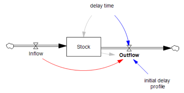
In Vensim, the conveyor is not really a distinct object in the language, which makes things better in one respect but worse in several others. The conveyor really lives in a function, DELAY CONVEYOR, which is used in the outflow. This means that the connection between the delay time parameter is properly both dynamic (for determining the outflow) and static (for initialization of the stock). However, the initial delay profile parameter is connected to the flow, not the stock, which is weird – this is because the stock is actually an accounting variable that is needed to keep track of the conveyor contents, rather than an actual dynamic participant in the structure, hence the lack of an arrow from stock to flow, except for initialization (gray). This convention also requires the oddity of a flow-to-flow connection (red) which is normally a no-no.

Similar problems exist for leakage flows, but I won’t detail those.

My conclusion is that both approaches are flawed. They both work mathematically, but neither portrays what’s really going on for the diagram viewer. We’ll get it right in a forthcoming version of Ventity, and maybe improve Vensim at some point.

Critiques of SD

I was flipping through the SD Discussion List archive and ran across this gem from George Richardson, responding to Bernadette O’Regan’s query about critiques of SD:

The significant or well-known criticisms of system dynamics include:

William Nordhaus, Measurement without Data (The Economic Journal, 83,332;
Dec. 1973)

[Nordhaus objects to the fact that Forrester seriously proposes a
world model fit to essentially only two data points. He simplifies the
model to help him analyze it, carries through some investigations that
cause him to doubt the model, and makes the mistake of critiquing a
univariate relation (effect of material standard of living on births)
using multivariate real world data — the real-world data has all the
other influences in the system at work, while Nordhaus wants to pull out
just the effect of standard of living). Sadly, a very influential
critique in the economics literature.]

See Forrester’s response in Jay. W. Forrester, Gilbert W. Low, and
Nathaniel J. Mass, The Debate on World Dynamics: a Response to Nordhaus
(Policy Sciences 5 (1974)
.

Joseph Weizenbaum, Computer Power and Human Reason (W.H. Freeman, 1976).
[Weizenbaum, a professor of computer science at MIT, was the author of
the speech processing and recognition program ELIZA. He became very
distressed at what people were proposing we could do with computers (e.g.,
use ELIZA seriously to counsel emotionally disturbed people), and wrote
this impassioned book about what in his view computers can do well and
what they cant. Contains sections on system dynamics in various places
and finds Forrester’s claims for the approach to be too broad and, like
Herbert Simon’s, “very simple.”]

Robert Boyd, World Dynamics: A Note (Science, 177, August 11, 1972).
[Boyd’s very original and interesting critique of World Dynamics tries
to use Forrester’s model itself to argue that World Dynamics did not solve
the essential question about limits to growth — whether technology can
avert the limits explicitly assumed in World Dynamics and the Limits to
Growth models. Boyd adds a Technology level to World Dynamics and
incorporates four effects on things like pollution generated per capita,
and finds that one can incorporate assumptions in the model that make the
problem go away. Unfortunately for his argument, Boyd’s additions are
extremely sensitive to particular parameter values and he unrealistically
assumes things like the second law of thermodynamics doesn’t apply. We
used to give this as an exercise: step 1 — build Boyd’s additions into
Forrester’s model and investigate; step 2 — incorporate Boyd’s
assumptions in Forrester’s original model just by changing parameters;
step 3 — reflect on what you’ve learned. Still a great exercise.]

Robert M. Solow, Notes on Doomsday Models (Proceedings of the National
Academy of Science 69,12, pp. 3832-3833, dec. 1972)
.
[Solow, an Institute Professor at MIT, critiqued the World Dynamics and
Limits to Growth models on structure (saying their conclusions were built
in), absence of a price system, and poor-to-nonexistent empirical
foundation. The differences between an econometric approach and a system
dynamics approach are quite vivid in this critique.]

H. Igor Ansoff and Dennis Slevin, An Appreciation of Industrial Dynamics.
(Management Science, 14,7, March 1968)
.
[Unfortunately, I no longer have a copy of this critique, so I cant
summarize it, but its worth finding in a library. See also Forrester’s
“A Response to Ansoff and Slevin” which also appeared in Management
Science (vol. 14, 9m May 1968)
, and is reprinted in Forrester’s Collected
Papers, available from Productivity Press.]

These are all rather ancient, “classical” critiques. I am not really
familiar with current critiques, either because they exist but have not
come to my attention or because they are few and far between. If the
latter, that could be because we are doing less controversial work these
days or because the critics think we’re not really a threat anymore.

I hope we’re still a threat.

…GPR


George P. Richardson
Rockefeller College of Public Affairs and Policy, SUNY, Albany

I’ll add a few more when I get a chance. These critiques really concern World Dynamics and the Limits to Growth rather than SD per se, but many have thrown the baby out with the bathwater. Some of these critiques have not aged well. But some are also still true. For example, Solow’s critique of World Dynamics starts with the absence of a price system, and Boyd’s critique center’s on the absence of technology. There are lots of SD models with prices and technology in them, but there isn’t really a successor to World Dynamics or World3 that does a good job of addressing these critiques. At the same time, I think it’s now obvious that neither prices nor technology has brought stability to the environment and resources.

Shoehorning the Problem into the Archetype

Barry Richmond in 1994, describing one of the hazards of archetypes:

The second practice we need to exercise great care in executing is the purveyance of “Systems Archetypes” (Senge, 1990). The care required becomes multiplied several-fold when these archetypes are packaged for consumption via causal loop diagrams. Again, to me, one of the major “problems” with System Dynamics was the “we have a way to get the wisdom, we’ll get it, then we’ll share it with you” orientation. I feel that Systems Thinking should be about helping to build people’s capacity for generating wisdom for themselves. Though I believe that Senge offered the archetypes in this latter spirit, too many people are taking them as “revealed truth,” looking for instances of that truth in their organizations (i.e., engaging in what amounts to a “matching exercise”), and calling this activity Systems Thinking. It isn’t. I have encountered many situations in which the result of pursuing this approach has left people feeling quite disenchanted with what they perceive Systems Thinking to be. This is not a “cheap shot” at Peter. His book has raised the awareness with respect to Systems Thinking for many people around the globe. However, we all need to exercise great caution in the purveyance of Systems Archetypes – in particular when that purveyance makes use of causal loop diagrams.

I’ve seen the problem of the “matching exercise” in classroom settings but not real projects. In practical settings, I do see some utility to the use of archetypes as a compact way to communicate among people familiar with the required systems lingo. In my view the real challenge is that archetypes are underspecified (compared to a simulation model), and therefore ambiguous. You can’t really tell by looking at the structure of a CLD what behavior will emerge. However, if you simulate a model, you might quickly realize, “hey, this is eroding goals” which could convey a whole package of ideas to your systems-aware colleagues.

What is SD? 2.0

I’ve just realized that I never followed up on my What is SD post to link in subsequent publication of the paper and 5 commentaries (including mine) in the System Dynamics Review.

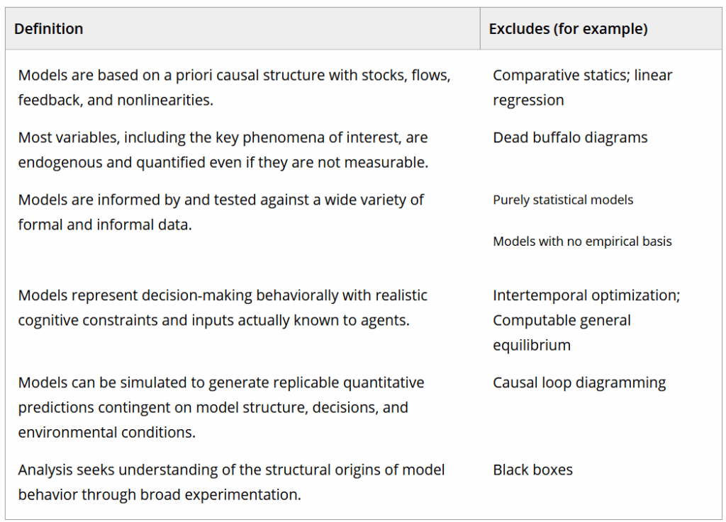
To summarize, the Naugle/Langarudi/Clancy proposal is:

  1. Models are based on causal feedback structure.
  2. Accumulations and delays are foundational.
  3. Models are equation-based.
  4. Concept of time is continuous.
  5. Analysis focuses on feedback dynamics.

My take is:

Interestingly, I think I’ve already violated at least two of my examples (more on that another time). I guess I contain multitudes.

The other commentaries each raise interesting points about the definition as well as the very idea of defining.

This topic came to mind because I rediscovered an old Barry Richmond article that also probes the definition of SD. Interestingly it slipped through the cracks and wasn’t cited by any of us (theoretically it was delivered at the ’94 SD conference, but it’s not in the proceedings).

System Dynamics/Systems Thinking: Let’s Just Get On With It

What is Systems Thinking, and how does it relate to System Dynamics? Let me begin by briefly saying what Systems Thinking is not. Systems Thinking is not General Systems Theory, nor is it “Soft Systems” or Systems Analysis – though it shares elements in common with all of these. Furthermore, Systems Thinking is not the same thing as Chaos Theory, Dissipative Structures, Operations Research, Decision Analysis, or what control theorists mean when they say System Dynamics – though, again, there are similarities both in subject matter and aspects of the associated methodologies. Nor is Systems Thinking hexagrams, personal mastery, dialogue, or total quality.

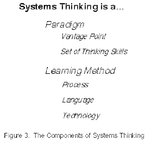
The definition of Systems Thinking at which I have arrived is: Systems Thinking is the art and science of making reliable inferences about behavior by developing an increasingly deep understanding of underlying structure. The art and science is composed of the pieces which are summarized in Figure 3.

I find Barry’s definition to be a particularly pithy elevator pitch for SD – I’m going to use it.

Tariff dumbnamics in the penguin island autarky

The formula behind the recent tariffs has spawned a lot of analysis, presumably because there’s plenty of foolishness to go around. Stand Up Maths has a good one:

I want to offer a slightly different take.

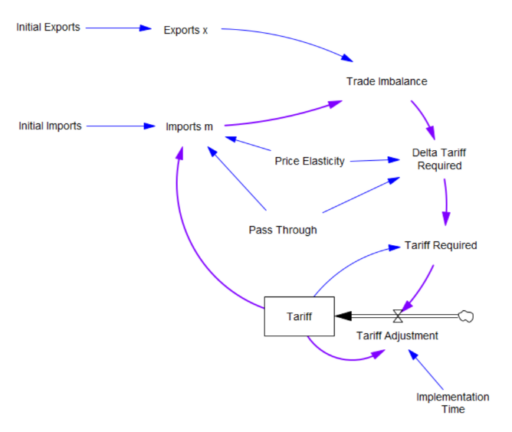
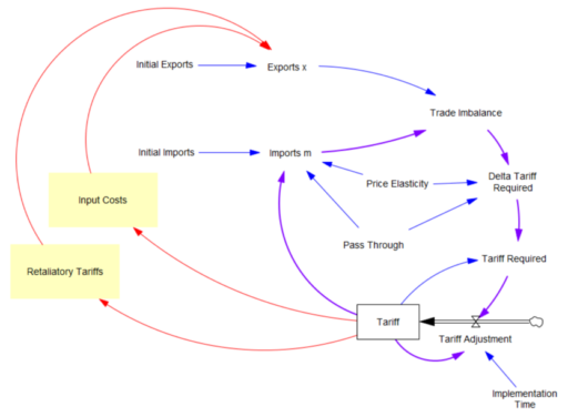
What the tariff formula is proposing is really a feedback control system. The goal of the control loop is to extinguish trade deficits (which the administration mischaracterized as “tariffs other countries charge us”). The key loop is the purple one, which establishes the tariff required to achieve balance:

The Tariff here is a stock, because it’s part of the state of the system – a posted price that changes in response to an adjustment process. That process isn’t instantaneous, though it seems that the implementation time is extremely short recently.

In this simple model, delta tariff required is the now-famous formula. There’s an old saw, that economics is the search for an objective function that makes revealed behavior optimal. There’s something similar here, which is discovering the demand function for imports m that makes the delta tariff required correct. There is one:

Imports m = Initial Imports*(1-Tariff*Pass Through*Price Elasticity)

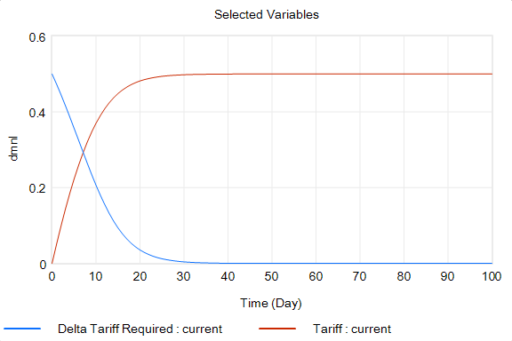
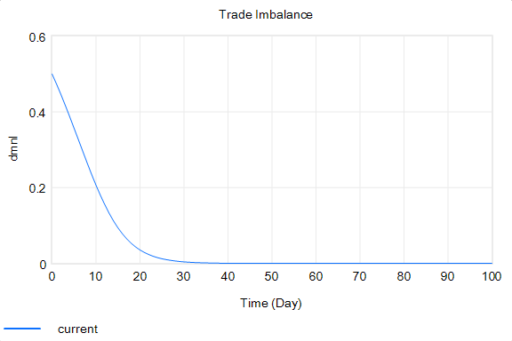
With that, the loop works exactly as intended: the tariff rises to the level predicted by the initial delta, and the trade imbalance is extinguished:

So in this case, the model produces the desired behavior, given the assumptions. It just so happens that the assumptions are really dumb.

You could quibble with the functional form and choice of parameters (which the calculation note sources from papers that don’t say what they’re purported to say). But I think the primary problem is omitted structure.

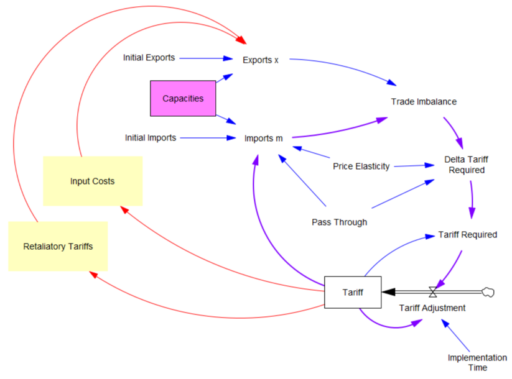
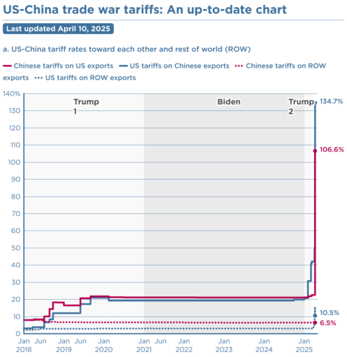
First, in the original model, exports are invariant. That’s obviously not the case, because (a) the tariff increases domestic costs, and therefore export prices, and (b) it’s naive to expect that other countries won’t retaliate. The escalation with China is a good example of the latter.

Second, the prevailing mindset seems to be that trade imbalances can adjust quickly. That’s bonkers. The roots of imbalances are structural, and baked in to the capacity of industries to produce and transport particular mixes of goods (pink below). Turning over the capital stocks behind those capacities takes years. Changing the technology and human capital involved might take even longer. A whole industrial ecosystem can’t just spring up overnight.

Third, in theory exchange rates are already supposed to be equilibrating trade imbalances, but they’re not. I think this is because they’re tied up with monetary and physical capital flows that aren’t in the kind of simple Ricardian barter model the administration is assuming. Those are potentially big issues, for which there isn’t good agreement about the structure.

I think the problem definition, boundary and goal of the system also need to be questioned. If we succeed in balancing trade, other countries won’t be accumulating dollars and plowing them back into treasuries to finance our debt. What will the bond vigilantes do then? Perhaps we should be looking to get our own fiscal house in order first.

Lately I’ve been arguing for a degree of predictability in some systems. However, I’ve also been arguing that one should attempt to measure the potential predictability of the system. In this case, I think the uncertainties are pretty profound, the proposed model has zero credibility, and better models are elusive, so the tariff formula is not predictive in any useful way. We should be treading carefully, not swinging wildly at a pinata where the candy is primarily trading opportunities for insiders.

Communicating uncertainty and policy sensitivity

This video is a quick attempt to run through some ways to look at how policy effects are contingent on an uncertain landscape.

I used a simple infection model in Ventity for convenience, though you could do this with many tools.

To paraphrase Mark Twain (or was it …), “If I had more time, I would have made a shorter video.” But that’s really part of the challenge: it’s hard to do a good job of explaining the dynamics of a system contingent on a wide variety of parameter choices in a short time.

One possible response is Forrester’s: we simply can’t teach everything about a nonlinear dynamic system if we have to start from scratch and the listener has a short attention span. So we need to build up systems literacy for the long haul. But I’d be interested in your thoughts on how to pack the essentials into a YouTube short.

Sources of Uncertainty

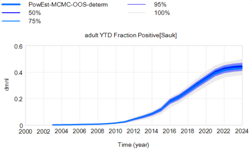
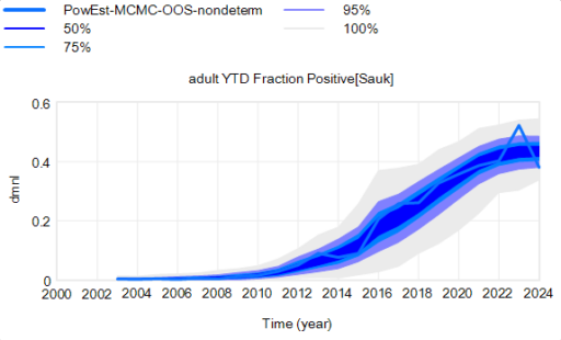
The confidence bounds I showed in my previous post have some interesting features. The following plots show three sources of the uncertainty in simulated surveillance for Chronic Wasting Disease in deer.

  • Parameter uncertainty
  • Sampling error in the measurement process
  • Driving noise from random interactions in the population

You could add external disturbances like weather to this list, though we don’t simulate it here.

By way of background, this come from a fairly big model that combines the dynamics of the host (deer) with an SIR-like model of disease transmission and progression. There’s quite a bit of disaggregation (regions, ages, sexes). The model is driven by historic harvest and sample sizes, and generates deer population, vegetation, and disease dynamics endogenously. The parameters used here represent a Bayesian posterior, from MCMC with literature priors and a lot of data. The parameter sample from the posterior is a joint distribution that captures both individual parameter variation and covariation (though with only a few exceptions things seem to be relatively independent).

Here’s the effect of parameter uncertainty on the disease trajectory:

Each of the 10,000 runs making up this ensemble is deterministic. It’s surprisingly tight, because it is well-determined by the data.

However, parameter uncertainty is not the only issue. Even if you know the actual state of the disease perfectly, there’s still uncertainty in the reported outcome due to sampling variation. You might stray from the “true” prevalence of the disease because of chance in the selection of which deer are actually tested. Making sampling stochastic broadens the bounds:

That’s still not the whole picture, because deer aren’t really deterministic. They come in integer quanta and they have random interactions. Thus a standard SD formulation like:

births = birth rate * doe population

becomes

births = Poisson( birth rate * doe population )

For stock outflows, like the transition from healthy to infected, the Binomial distribution may be the appropriate choice. This randomness in flows means there’s additional variance around the deterministic course, and the model can explore a wider set of trajectories.

There’s one other interesting feature, particularly evident in this last graph: uncertainty around the mean (i.e. the geometric standard deviation) varies quite a bit. Initially, uncertainty increases with time – as Yogi Berra said, “It’s tough to make predictions, especially about the future.” In the early stages of the disese (2003-2008 say), numbers are small and random events affect the timing of takeoff of the disease, amplified by future positive feedback. A deterministic disease model with reproduction ratio R0>1 can only grow, but in a stochastic model luck can cause the disease to go extinct or bumble around 0 prevalence for a while before emerging into growth. Towards the end of this simulation, the confidence bounds narrow. There are two reasons for this: negative feedback is starting to dominate as the disease approaches saturation prevalence, and at the same time the normalized standard deviation of the sampling errors and randomness in deer dynamics is decreasing as the numbers become larger (essentially with 1/sqrt(n)).

This is not uncommon in real systems. For example, you may be unsure where a chaotic pendulum will be in it’s swing a minute from now. But you can be pretty sure that after an hour or a day it will be hanging idle at dead center. However, this might not remain true when you broaden the boundary of the system to include additional feedbacks or disturbances. In this CWD model, for example, there’s some additional feedback from human behavior (not in the statistical model, but in the full version) that conditions the eventual saturation point, perhaps preventing convergence of uncertainty.