Exploring stimulus policy

To celebrate the debt ceiling deal, I updated my copy of Nathan Forrester’s model, A Dynamic Synthesis of Basic Macroeconomic Theory.

Now, to celebrate the bad economic news and increasing speculation of a double-dip depression replay, here are some reflections on policy, using that model.

The model combines a number of macro standards: the multiplier-accelerator, inventory adjustment, capital accumulation, the IS-LM model, aggregate supply/aggregate demand dynamics, the permanent income hypothesis and the Phillips curve.

Forrester experimented with the model to identify the effects of five policies intended to stabilize fluctuations: countercyclical government transfers and spending, graduated income taxes, and money supply growth or targets. He used simulations experiments and linear system analysis (frequency response and eigenvalue elasticity) to identify the contribution of policies to stability.

Interestingly, the countercyclical policies tend to destabilize the business cycle. However, they prove to be stabilizing for a long-term cycle associated with the multiplier-accelerator and involving capital stock and long-term expectations.

I got curious about the effect of these policies through a simulated recession like the one we’re now in. So, I started from equilibrium and created a recession by imposing a negative shock to final sales, which passes immediately into aggregate demand. Here’s what happens:

There’s a lot of fine detail, so you may want to head over to Vimeo to view in full screen HD.

This is part of a couple of experiments I’ve tried with screencasting models, as practice for creating some online Vensim training materials. My preliminary observation is that even a perfunctory exploration of a simple model is time consuming to create and places high demands on audience attention. It’s no wonder you never see any real data or math on the Discovery Channel. I’d be interested to hear of examples of this sort of thing done well.

Thinking about stuff

A while back I decided to never buy another garden plant unless I’d first dug the hole for it. In a single stroke, this simple rule eliminated impulse shopping at the nursery, improved the survival rate of new plants, and increased overall garden productivity.

This got me thinking about the insidious dynamics of stuff, by which tools come to rule their masters. I’ve distilled most of my thinking into this picture:


Click to enlarge.

This is mainly a visual post, but here’s a quick guide to some of the loops:

Black: stuff is the accumulation of shopping, less outflows from discarding and liquidation.

Red: Shopping adjusts the stock of stuff to a goal. The goal is set by income (a positive feedback, to the extent that stuff makes you more productive, so you can afford more stuff) and by the utility of stuff at the margin, which falls as you have less and less time to use each item of stuff, or acquire increasingly useless items.

So far, Economics 101 would tell a nice story of smooth adjustment of the shopping process to an equilibrium at the optimal stuff level. That’s defeated by the complexity of all of the other dynamics, which create a variety of possible vicious cycles and misperceptions of feedback that result in suboptimal stuffing.

Orange: You need stuff to go with the stuff. The iPad needs a dock, etc. Even if the stuff is truly simple, you need somewhere to put it.

Green: Society reinforces the need for stuff, via keep-up-with-the-Joneses and neglect of shared stuff. When you have too much stuff, C.H.A.O.S. ensues – “can’t have anyone over syndrome” – which reinforces the desire for stuff to hide the chaos or facilitate fun without social contact.

Blue: Stuff takes time, in a variety of ways. The more stuff  you have, the less time you actually have for using stuff for fun. This can actually increase your desire for stuff, due to the desire to have fun more efficiently in the limited time available.

Brown: Pressure for time and more stuff triggers a bunch of loops involving quality of stuff. One response is to buy low-quality stuff, which soon increases the stock of broken stuff lying about, worsening time pressure. One response is the descent into disposability, which saves the time, at the expense of a high throughput (shopping->discarding) relative to the stock of stuff. Once you’re fully stocked with low-quality stuff, why bother fixing it when it breaks? Fixing one thing often results in collateral damage to another (computers are notorious for this).

I’m far from a successful minimalist yet, but here’s what’s working for me to various degrees:

  • The old advice, “Use it up, wear it out, make it do or do without” works.
  • Don’t buy stuff when you can rent it. Unfortunately rental markets aren’t very liquid so this can be tough.
  • Allocate time to liquidating stuff. This eats up free time in the short run, but it’s a worse-before-better dynamic, so there’s a payoff in the long run. Fortunately liquidating stuff has a learning curve – it gets easier.
  • Make underutilized and broken stuff salient, by keeping lists and eliminating concealing storage.
  • Change your shopping policy to forbid acquisition of new stuff until existing stuff has been dealt with.
  • Buy higher quality than you think you’ll need.
  • Learn low-stuff skills.
  • Require steady state stuff: no shopping for new things until something old goes to make way for it.
  • Do things, even when you don’t have the perfect gear.
  • Explicitly prioritize stuff acquisition.
  • Tax yourself, or at least mentally double the price of any proposed acquisition, to account for all the side effects that you’ll discover later.
  • Get relatives to give $ to your favorite nonprofit rather than giving you something you won’t use.

There are also some policies that address the social dimensions of stuff:

  • Underdress and underequip. Occasionally this results in your own discomfort, but reverses the social arms race.
  • Don’t reward other peoples’ shopping by drooling over their stuff. Pity them.
  • Use and promote shared stuff, like parks.

This system has a lot of positive feedback, so once you get the loops running the right way, improvement really takes off.

The rise of systems sciences

The Google books ngram viewer nicely documents the rise of various systems science disciplines, from about the time of Maxwell’s landmark 1868 paper, On Governors:

Click to enlarge.

We still have a long way to go though:

Further reading:

Limits to bathtubs

Danger lurks in the bathtub – not just slips, falls, and Norman Bates, but also bad model formulations.

A while ago, after working with my kids to collect data on our bathtub, I wrote My bathtub is nonlinear.

We grabbed a sheet of graph paper, fat pens, a yardstick, and a stopwatch and headed for the bathtub. …

When the tub was full, we made a few guesses about how long it might take to empty, then started the clock and opened the drain. Every ten or twenty seconds, we’d stop the timer, take a depth reading, and plot the result on our graph. …

To my astonishment, the resulting plot showed a perfectly linear decline in water depth, all the way to zero (as best we could measure). In hindsight, it’s not all that strange, because the tub tapers at the bottom, so that a constant linear decline in the outflow rate corresponds with the declining volumetric flow rate you’d expect (from decreasing pressure at the outlet as the water gets shallower). Still, I find it rather amazing that the shape of the tub (and perhaps nonlinearity in the drain’s behavior) results in such a perfectly linear trajectory.

It turns out that my attribution of the linear time vs. depth profile was sloppy – the behavior has a little to do with tub shape, and a lot to do with nonlinearity in the draining behavior. In a nice brief from the SD conference, Pål Davidsen, Erling Moxnes, Mauricio Munera Sánchez and David Wheat explain why:

… in the 16th century the Italian scientist Evangelista Torricelli found the relationship between water height and outflow to be nonlinear.

… Torricelli may have reasoned as follows. Let a droplet of water fall frictionless outside the tank from the same height … as the surface of the water. Gravitation will make the droplet accelerate. As the droplet passes the bottom of the tank, its kinetic energy will equal the loss of potential energy … Reorganizing this equation Torricelli found the following nonlinear expression for speed as a function of height

v = SQRT(2*g*h)

Then Torricelli moved inside the tank and reasoned that the same must apply there. …

Assuming that the water tank is a cylinder with straight walls … The outflow is given by the square root of volume; it is not a linear function of volume.

– “A note on the bathtub analogy,” ISDC 2011; final proceedings aren’t online yet but presumably will be here eventually.

In hindsight, this ought to have been obvious to me, because bathtubs clearly don’t exhibit the heavy-right-tail behavior of a first order linear draining process. The difference matters:

The bathtub analogy has been used extensively to illustrate stock and flow relationships. Because this analogy is frequently used, System Dynamicists should be aware that the natural outflow of water from a bathtub is a nonlinear function of water volume. A questionnaire suggests that students with one year or more of System Dynamics training tend to assume a linear relationship when asked to model a water outflow driven by gravity. We present Torricelli’s law for the outflow and investigate the error caused by assuming linearity. We also construct an “inverted funnel” which does behave like a linear system. We conclude by pointing out that the nonlinearity is of no importance for the usefulness of bathtubs or funnels as analogies. On the other hand, simplified analogies could make modellers overconfident in linear formulations and not able to address critical remarks from physicists or other specialists.

I’ve been doing SD for over two decades, and have the physical science background to know better, but found it a little too easy to assume a linear bathtub as a mental model, without inquiring very deeply when confronted with disconfirming data. For me, this is a nice cautionary lesson, that we forget the roots of system dynamics in engineering at our own peril.

My implementation of the model is in my library.

Is London a big whale?

Why do cities survive atom bombs, while companies routinely go belly up?

Geoffrey West on The Surprising Math of Cities and Corporations:

There’s another interesting video with West in the conversations at Edge.

West looks at the metabolism of cities, and observes scale-free behavior of good stuff (income, innovation, input efficiency) as well as bad stuff (crime, disease – products of entropy). The destiny of cities, like companies, is collapse, except to the extent that they can innovate at an accelerating rate. Better hope the Singularity is on schedule.

Thanks to whoever it was at the SD conference who pointed this out!

Modeling is not optional

EVERY GOOD REGULATOR OF A SYSTEM MUST BE A MODEL OF THAT SYSTEM

The design of a complex regulator often includes the making of a model of the system to be regulated. The making of such a model has hitherto been regarded as optional, as merely one of many possible ways.

In this paper a theorem is presented which shows, under very broad conditions, that any regulator that is maximally both successful and simple must be isomorphic with the system being regulated.  (The exact assumptions are given.) Making a model is thus necessary.

The theorem has the interesting corollary that the living brain, so far as it is to be successful and efficient as a regulator for survival, must proceed, in learning, by the formation of a model (or models) of its environment.

That’s from a classic cybernetics paper by Conant & Ashby (Int. J. Systems Sci., 1970, vol. 1, No. 2, 89-97). It even has an interesting web project dedicated to it.

It’s one of several on a nice reading list on the foundations of complexity that I ran across at the Sante Fe Institute. Some of the pdfs are here.

Drunker than intended and overinvested

Erling Moxnes on the dangers of forecasting without structural insight and the generic structure behind getting too drunk and underestimating delays when investing in a market, with the common outcome of  instability.

More on drinking dynamics here, implemented as a game on Forio (haven’t tried it yet – curious about your experience if you do).

Setting up Vensim compiled simulation on Windows

If you don’t use Vensim DSS, you’ll find this post rather boring and useless. If you do, prepare for heart-pounding acceleration of your big model runs:

  • Get Vensim DSS.
  • Get a C compiler. Most flavors of Microsoft compilers are compatible; MS Visual C++ 2010 Express is a good choice (and free). You could probably use gcc, but I’ve never set it up. I’ve heard reports of issues with 2005 and 2008 versions, so it may be worth your while to upgrade.
  • Install Vensim, if you haven’t already, being sure to check the Install external function and compiled simulation support box.
  • Launch the program and go to Tools>Options…>Startup and set the Compiled simulation path to C:Documents and SettingsAll UsersVensimcomp32 (WinXP) or C:UsersPublicVensimcomp32 (Vista/7).
    • Check your mdl.bat in the location above to be sure that it points to the right compiler. This is a simple matter of checking to be sure that all options are commented out with “REM ” statements, except the one you’re using, for example:
  • Move to the Advanced tab and set the compilation options to Query or Compile (you may want to skip this for normal Simulation, and just do it for Optimization and Sensitivity, where speed really counts).

This is well worth the hassle if you’re working with a large model in SyntheSim or doing a lot of simulations for sensitivity analysis and optimization. The speedup is typically 4-5x.

Elk, wolves and dynamic system visualization

Bret Victor’s video of a slick iPad app for interactive visualization of the Lotka-Voltera equations has been making the rounds:

Coincidentally, this came to my notice around the same time that I got interested in the debate over wolf reintroduction here in Montana. Even simple models say interesting things about wolf-elk dynamics, which I’ll write about some other time (I need to get vaccinated for rabies first).

To ponder the implications of the video and predator-prey dynamics, I built a version of the Lotka-Voltera model in Vensim.

After a second look at the video, I still think it’s excellent. Victor’s two design principles, ubiquitous visualization and in-context manipulation, are powerful for communicating a model. Some aspects of what’s shown have been in Vensim since the introduction of SyntheSim a few years ago, though with less Tufte/iPad sexiness. But other features, like Causal Tracing, are not so easily discovered – they’re effective for pros, but not new users. The way controls appear at one’s fingertips in the iPad app is very elegant. The “sweep” mode is also clever, so I implemented a similar approach (randomized initial conditions across an array dimension) in my version of the model. My favorite trick, though, is the 2D control of initial conditions via the phase diagram, which makes discovery of the system’s equilibrium easy.

The slickness of the video has led some to wonder whether existing SD tools are dinosaurs. From a design standpoint, I’d agree in some respects, but I think SD has also developed many practices – only partially embodied in tools – that address learning gaps that aren’t directly tackled by the app in the video: Continue reading “Elk, wolves and dynamic system visualization”

Who moved my eigenvalues?

Change management is one of the great challenges in modeling projects. I don’t mean this in the usual sense of getting people to change on the basis of model results. That’s always a challenge, but there’s another.

Over the course of a project, the numerical results and maybe even the policy conclusions given by a model are going to change. This is how we learn from models. If the results don’t change, either we knew the answer from the outset (a perception that should raise lots of red flags), or the model isn’t improving.

The problem is that model consumers are likely to get anchored to the preliminary results of the work, and resist change when it arrives later in the form of graphs that look different or insights that contradict early, tentative conclusions.

Fortunately, there are remedies:

  • Start with the assumption that the model and the data are wrong, and to some extent will always remain so.
  • Recognize that the modeler is not the font of all wisdom.
  • Emphasize extreme conditions tests and reality checks throughout the modeling process, not just at the end, so bugs don’t get baked in while insights remain hidden.
  • Do lots of sensitivity analysis to determine the circumstances under which insights are valid.
  • Keep the model simpler than you think it needs to be, so that you have some hope of understanding it, and time for reflecting on behavior and communicating results.
  • Involve a broad team of model consumers, and set appropriate expectations about what the model will be and do from the start.