Don't just do something, stand there! Reflections on the counterintuitive behavior of complex systems, seen through the eyes of System Dynamics, Systems Thinking and simulation.
I’ve just realized that I never followed up on my What is SD post to link in subsequent publication of the paper and 5 commentaries (including mine) in the System Dynamics Review.
Interestingly, I think I’ve already violated at least two of my examples (more on that another time). I guess I contain multitudes.
The other commentaries each raise interesting points about the definition as well as the very idea of defining.
This topic came to mind because I rediscovered an old Barry Richmond article that also probes the definition of SD. Interestingly it slipped through the cracks and wasn’t cited by any of us (theoretically it was delivered at the ’94 SD conference, but it’s not in the proceedings).
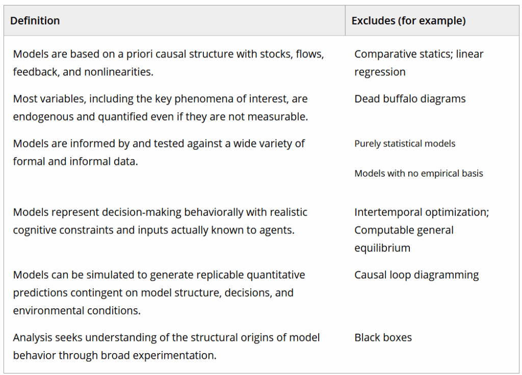
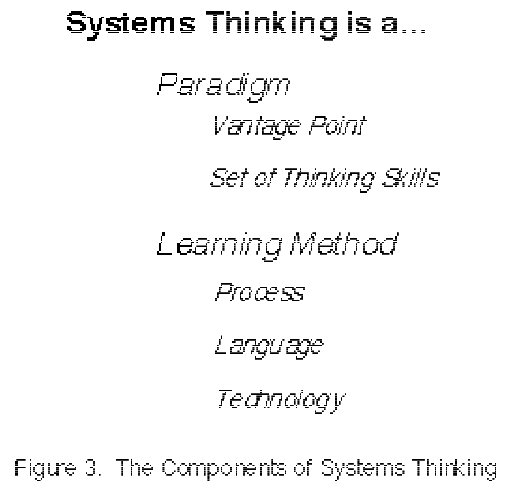
What is Systems Thinking, and how does it relate to System Dynamics? Let me begin by briefly saying what Systems Thinking is not. Systems Thinking is not General Systems Theory, nor is it “Soft Systems” or Systems Analysis – though it shares elements in common with all of these. Furthermore, Systems Thinking is not the same thing as Chaos Theory, Dissipative Structures, Operations Research, Decision Analysis, or what control theorists mean when they say System Dynamics – though, again, there are similarities both in subject matter and aspects of the associated methodologies. Nor is Systems Thinking hexagrams, personal mastery, dialogue, or total quality.
…
The definition of Systems Thinking at which I have arrived is: Systems Thinking is the art and science of making reliable inferences about behavior by developing an increasingly deep understanding of underlying structure. The art and science is composed of the pieces which are summarized in Figure 3.
I find Barry’s definition to be a particularly pithy elevator pitch for SD – I’m going to use it.
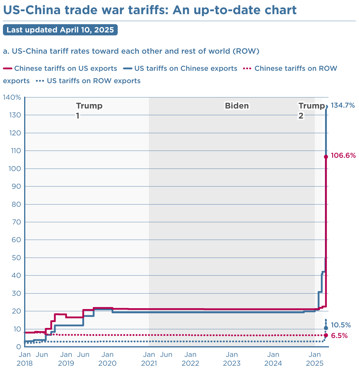
The formula behind the recent tariffs has spawned a lot of analysis, presumably because there’s plenty of foolishness to go around. Stand Up Maths has a good one:
I want to offer a slightly different take.
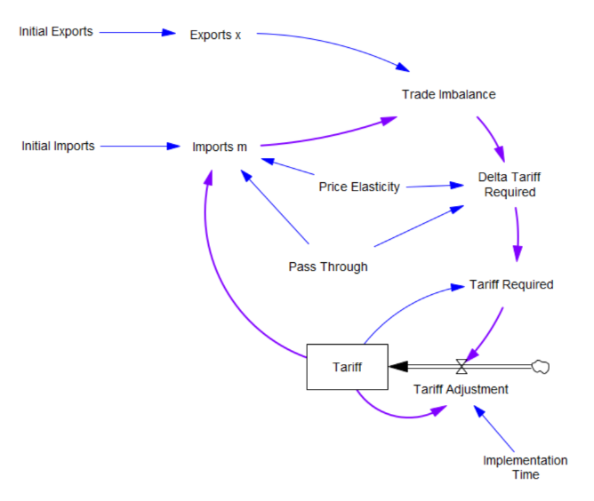
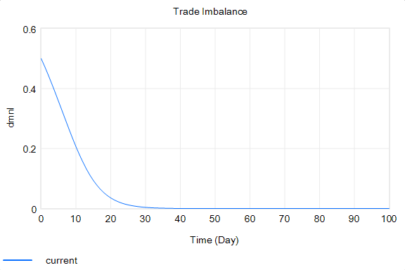
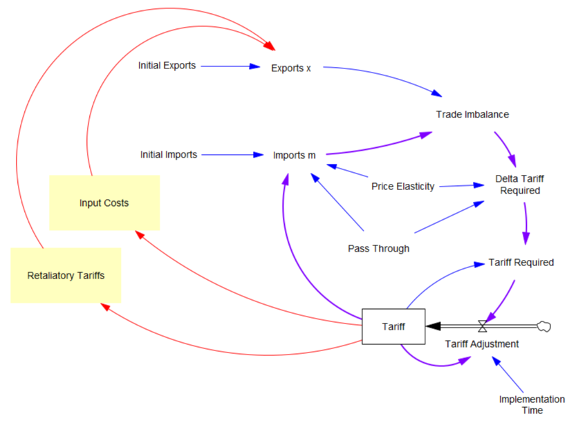
What the tariff formula is proposing is really a feedback control system. The goal of the control loop is to extinguish trade deficits (which the administration mischaracterized as “tariffs other countries charge us”). The key loop is the purple one, which establishes the tariff required to achieve balance:
The Tariff here is a stock, because it’s part of the state of the system – a posted price that changes in response to an adjustment process. That process isn’t instantaneous, though it seems that the implementation time is extremely short recently.
In this simple model, delta tariff required is the now-famous formula. There’s an old saw, that economics is the search for an objective function that makes revealed behavior optimal. There’s something similar here, which is discovering the demand function for imports m that makes the delta tariff required correct. There is one:
Imports m = Initial Imports*(1-Tariff*Pass Through*Price Elasticity)
With that, the loop works exactly as intended: the tariff rises to the level predicted by the initial delta, and the trade imbalance is extinguished: So in this case, the model produces the desired behavior, given the assumptions. It just so happens that the assumptions are really dumb.
You could quibble with the functional form and choice of parameters (which the calculation note sources from papers that don’t say what they’re purported to say). But I think the primary problem is omitted structure.
First, in the original model, exports are invariant. That’s obviously not the case, because (a) the tariff increases domestic costs, and therefore export prices, and (b) it’s naive to expect that other countries won’t retaliate. The escalation with China is a good example of the latter.
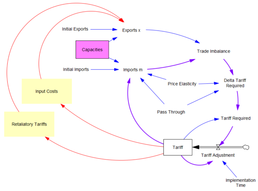
Second, the prevailing mindset seems to be that trade imbalances can adjust quickly. That’s bonkers. The roots of imbalances are structural, and baked in to the capacity of industries to produce and transport particular mixes of goods (pink below). Turning over the capital stocks behind those capacities takes years. Changing the technology and human capital involved might take even longer. A whole industrial ecosystem can’t just spring up overnight.
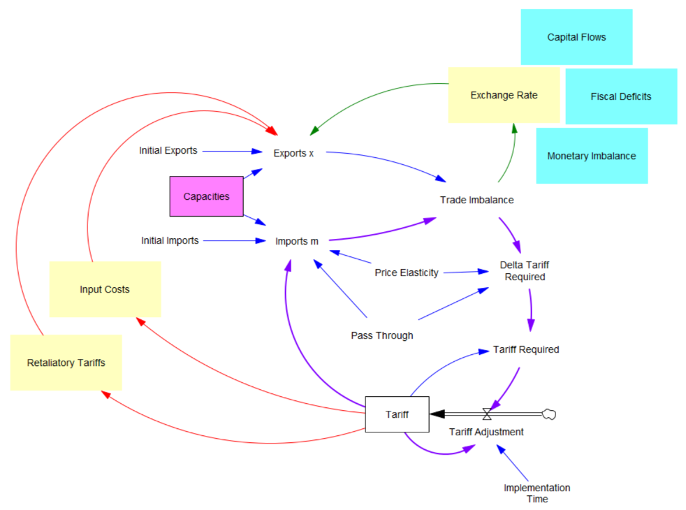
Third, in theory exchange rates are already supposed to be equilibrating trade imbalances, but they’re not. I think this is because they’re tied up with monetary and physical capital flows that aren’t in the kind of simple Ricardian barter model the administration is assuming. Those are potentially big issues, for which there isn’t good agreement about the structure.
I think the problem definition, boundary and goal of the system also need to be questioned. If we succeed in balancing trade, other countries won’t be accumulating dollars and plowing them back into treasuries to finance our debt. What will the bond vigilantes do then? Perhaps we should be looking to get our own fiscal house in order first.
Lately I’ve been arguing for a degree of predictability in some systems. However, I’ve also been arguing that one should attempt to measure the potential predictability of the system. In this case, I think the uncertainties are pretty profound, the proposed model has zero credibility, and better models are elusive, so the tariff formula is not predictive in any useful way. We should be treading carefully, not swinging wildly at a pinata where the candy is primarily trading opportunities for insiders.
This video is a quick attempt to run through some ways to look at how policy effects are contingent on an uncertain landscape.
I used a simple infection model in Ventity for convenience, though you could do this with many tools.
To paraphrase Mark Twain (or was it …), “If I had more time, I would have made a shorter video.” But that’s really part of the challenge: it’s hard to do a good job of explaining the dynamics of a system contingent on a wide variety of parameter choices in a short time.
One possible response is Forrester’s: we simply can’t teach everything about a nonlinear dynamic system if we have to start from scratch and the listener has a short attention span. So we need to build up systems literacy for the long haul. But I’d be interested in your thoughts on how to pack the essentials into a YouTube short.
It’s not necessarily true that what goes up must come down. Have we reached tariff orbital escape velocity? Or will the positive loops driving this reverse from vicious to virtuous cycle without some intervening catastrophe?
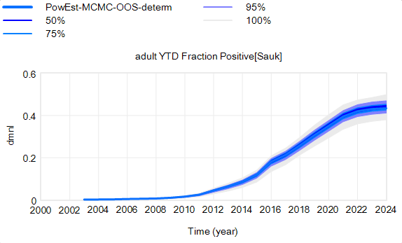
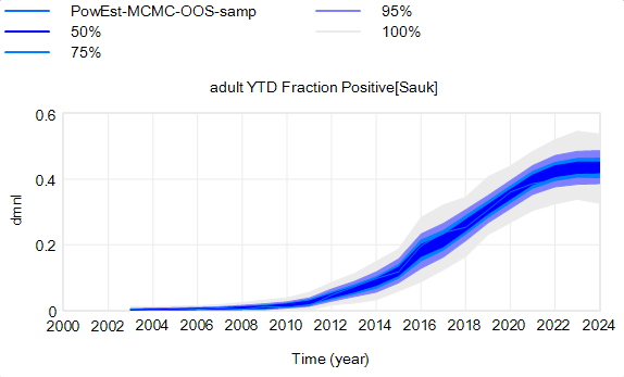
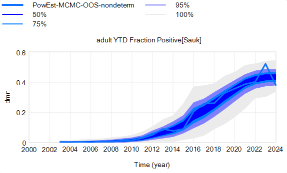
The confidence bounds I showed in my previous post have some interesting features. The following plots show three sources of the uncertainty in simulated surveillance for Chronic Wasting Disease in deer.
Parameter uncertainty
Sampling error in the measurement process
Driving noise from random interactions in the population
You could add external disturbances like weather to this list, though we don’t simulate it here.
By way of background, this come from a fairly big model that combines the dynamics of the host (deer) with an SIR-like model of disease transmission and progression. There’s quite a bit of disaggregation (regions, ages, sexes). The model is driven by historic harvest and sample sizes, and generates deer population, vegetation, and disease dynamics endogenously. The parameters used here represent a Bayesian posterior, from MCMC with literature priors and a lot of data. The parameter sample from the posterior is a joint distribution that captures both individual parameter variation and covariation (though with only a few exceptions things seem to be relatively independent).
Here’s the effect of parameter uncertainty on the disease trajectory:
Each of the 10,000 runs making up this ensemble is deterministic. It’s surprisingly tight, because it is well-determined by the data.
However, parameter uncertainty is not the only issue. Even if you know the actual state of the disease perfectly, there’s still uncertainty in the reported outcome due to sampling variation. You might stray from the “true” prevalence of the disease because of chance in the selection of which deer are actually tested. Making sampling stochastic broadens the bounds:
That’s still not the whole picture, because deer aren’t really deterministic. They come in integer quanta and they have random interactions. Thus a standard SD formulation like:
For stock outflows, like the transition from healthy to infected, the Binomial distribution may be the appropriate choice. This randomness in flows means there’s additional variance around the deterministic course, and the model can explore a wider set of trajectories.
There’s one other interesting feature, particularly evident in this last graph: uncertainty around the mean (i.e. the geometric standard deviation) varies quite a bit. Initially, uncertainty increases with time – as Yogi Berra said, “It’s tough to make predictions, especially about the future.” In the early stages of the disese (2003-2008 say), numbers are small and random events affect the timing of takeoff of the disease, amplified by future positive feedback. A deterministic disease model with reproduction ratio R0>1 can only grow, but in a stochastic model luck can cause the disease to go extinct or bumble around 0 prevalence for a while before emerging into growth. Towards the end of this simulation, the confidence bounds narrow. There are two reasons for this: negative feedback is starting to dominate as the disease approaches saturation prevalence, and at the same time the normalized standard deviation of the sampling errors and randomness in deer dynamics is decreasing as the numbers become larger (essentially with 1/sqrt(n)).
This is not uncommon in real systems. For example, you may be unsure where a chaotic pendulum will be in it’s swing a minute from now. But you can be pretty sure that after an hour or a day it will be hanging idle at dead center. However, this might not remain true when you broaden the boundary of the system to include additional feedbacks or disturbances. In this CWD model, for example, there’s some additional feedback from human behavior (not in the statistical model, but in the full version) that conditions the eventual saturation point, perhaps preventing convergence of uncertainty.
I posted my recent blogs on Forrester and forecasting uncertainty over at LinkedIn, and there’s been some good discussion. I want to highlight a few things.
First, a colleague pointed out that the way terms are understood is in the eye of the beholder. When you say “forecast” or “prediction” or “projection” the listener (client, stakeholder) may not hear what you mean. So regardless of whether your intention is correct when you say you’re going to “predict” something, you’d better be sure that your choice of language communicates to the end user with some fidelity.
Second, Samuel Allen asked a great question, which I haven’t answered to my satisfaction, “what are some good ways of preventing consumers of our conditional predictions from misunderstanding them?”
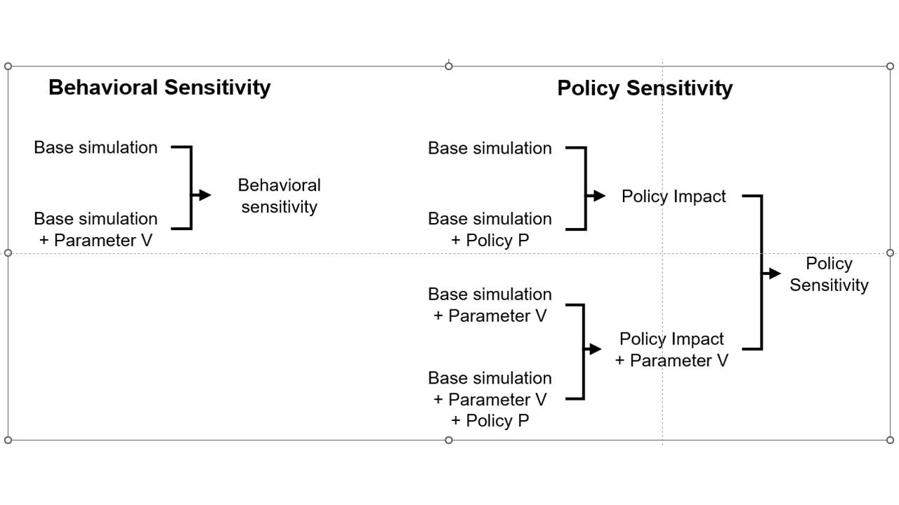
an explanation that has communicated well starts from the distinction between behavior sensitivity (does the simulation change?) versus outcome or policy sensitivity (does the size or direction of the policy impact change?). Two different sets of experiments are needed to answer the two different questions, which are visually distinct:
This is basically a cleaner explanation of what’s going on in my post on Forecasting Uncertainty. I think what I did there is too complex (too many competing lines), so I’m going to break it down into simpler parts in a followup.
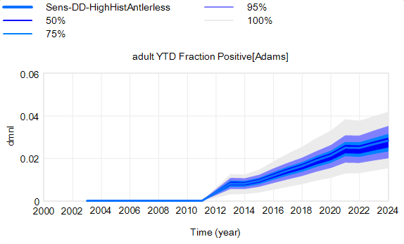
Another piece of the puzzle is visualization. Here’s a pair of scenarios from our CWD model. These are basically nowcasts showing uncertainty about historic conditions, subject to actual historic actions or a counterfactual “high harvest” scenario:
Note that I’m just grabbing raw stuff out of Vensim; for presentation these graphics could be cleaner. Also note the different scales.
On each of these charts, the spread indicates uncertainty from parameters and sampling error in disease surveillance. Comparing the two tells you how the behavior – including the uncertainty – is sensitive to the policy change.
In my experience, this works, but it’s cumbersome. There’s just too much information. You can put the two confidence bands on the same chart, using different colors, but then you have fuzzy things overlapping and it’s potentially hard to read.
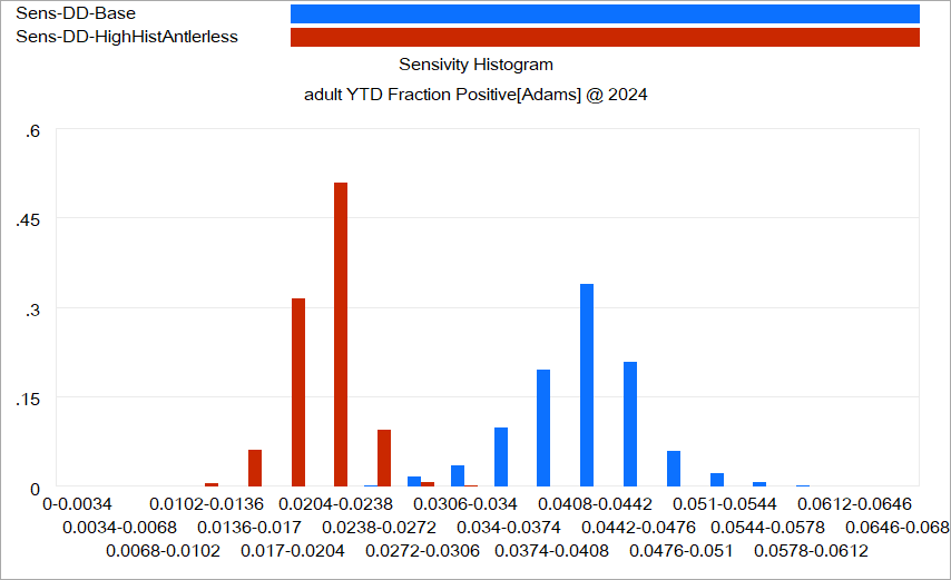
Another option is to use histograms that slice the outcome (here, at the endpoint):
Again, this is just a quick capture that could be improved with minimal effort. The spread for each color shows the distribution of possibilities, given the uncertainty from parameters and sampling. The spread between the colors shows the policy impact. You can see that the counterfactual policy (red) both improves the mean outcome (shift left) and reduces the variance (narrower). I actually like this view of things. Unfortunately, I haven’t had much luck with such things in general audiences, who tend to wonder what the axes represent.
I think one answer may be that you simply have to go back to basics and explore the sensitivity of the policy to individual parameter changes, in paired trials per Alan Graham’s diagram above, in order to build understanding of how this works.
I think the challenge of this task – and time required to address it – should not be underestimated. I think there’s often a hope that an SD model can be used to extract an insight about some key leverage point or feedback loop that solves a problem. With the new understanding in hand, the model can be discarded. I can think of some examples where this worked, but they’re mostly simple systems and one-off decisions. In complex situations with a lot of uncertainty, I think it may be necessary to keep the model in the loop. Otherwise, a year down the road, arrival of confounding results is likely to drive people back to erroneous heuristics and unravel the solution.
I’d be interested to hear success stories about communicating model uncertainty.
Here’s how SD modeling (and science generally) roughly works. Pick a question about a phenomenon of interest. Observe some stuff. Construct some mechanistic theories, what Barry Richmond called “operational thinking.” Test the theories against the observations, and reject or adapt the ones that don’t fit. Also test the theories for consistency with conservation laws, dimensional consistency, robustness in extreme conditions, and other things you know a priori from physics, adjacent models, or other levels of description. The quality of the model that survives is proportional to how hard you tried.
To verify what you’ve done, you either need to attempt to control the system according to your theory, or failing that, make some out of sample predictions and gather new data to see if they come true. This could mean replicating a randomized controlled trial, or predicting the future outcome of a change and waiting a while, or attempting to measure something not previously observed.
Now, if you think your mechanistic theories aren’t working, you can simply assert that the system is random, subject to acts of God, etc. But that’s a useless, superstitious, non-falsifiable and non-actionable statement, and you can’t beat something with nothing. In reality, any statement to the effect that “stuff happens” implies a set of possibilities that can be characterized as a null model with some implicit distribution.
If you’re doing something like a drug trial, the null hypothesis (no difference between drug and placebo) and statistics for assessing the actual difference are well known. Dynamic modeling situations are typically more complex and less controlled (i.e. observational), but that shouldn’t stop you. Suppose I predict that GDP/capita in the US will grow according to:
we could then compare outcomes. But first, we’d have to each specify the error bars around our prediction. If I’m confident, I might pick N(0,0.2%) and you argue for “stuff happens” at N(0,1%). If we evaluate next year, and growth is 1.8%, you seemingly win, because you’re right on the money, whereas my prediction (about 2%) is 1 standard deviation off. But not so fast … my prediction was 5x narrower. To decide who actually wins, we could look at the likelihood of each outcome.
My log-likelihood is (up to a constant):
-LN(.1)-(.2/.1)^2/2 = 0.39
Yours is:
-LN(1)-(0/.1)^2 = 0
So actually, my likelihood is bigger – I win. Your forecast happened to be right, but was so diffuse that it should be penalized for admitting a wide range of possible outcomes.
If this seems counterintuitive, consider a shooting contest. I propose to hit a bottle on a distant fencepost with my rifle. You propose to hit the side of a nearby barn with your shotgun. I only nick the bottle, causing it to wobble. You hit the barn. Who is the better shot?
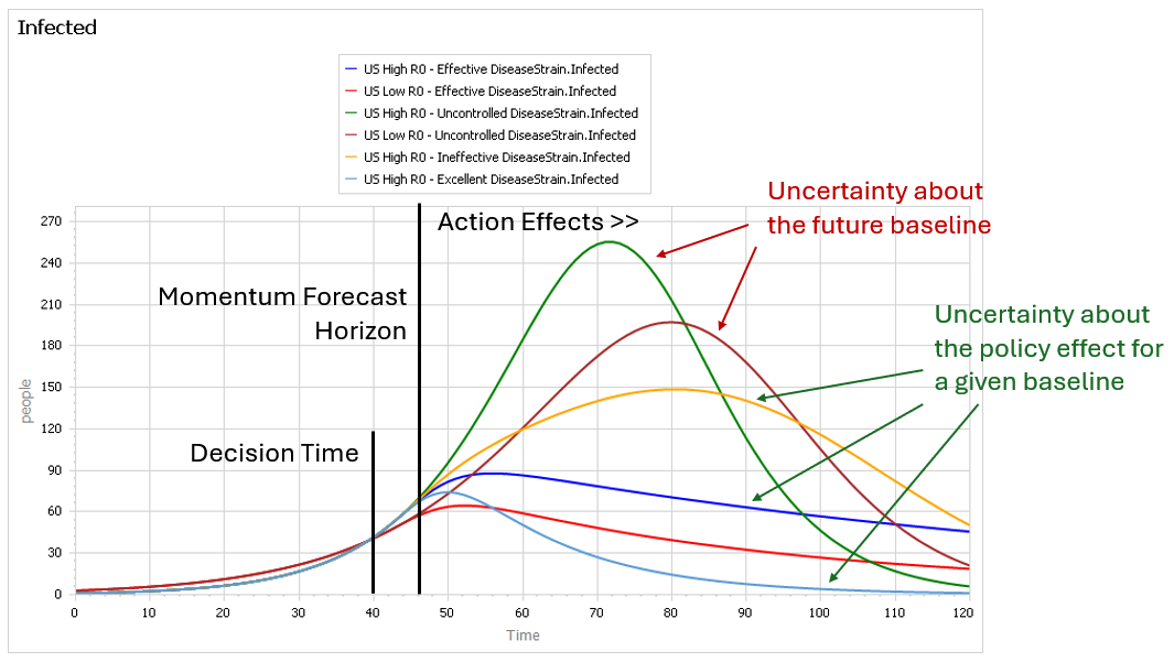
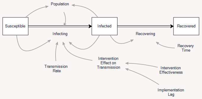
This is a set of scenarios from a simple SIR epidemic model in Ventity.
There are two sources of uncertainty in this model: the aggressiveness of the disease (transmission rate) and the effectiveness of an NPI policy that reduces transmission.
Early in the epidemic, at time 40 where the decision to intervene is made, it’s hard to tell the difference between a high transmission rate and a lower transmission rate with a slightly larger initial infected population. This is especially true in the real world, because early in an epidemic the information-gathering infrastructure is weak.
However, you can still make decent momentum forecasts by extrapolating from the early returns for a few more days – to time 45 or 50 perhaps. But this is not useful, because that roughly corresponds with the implementation lag for the policy. So, over the period of skilled momentum forecasts, it’s not possible to have much influence.
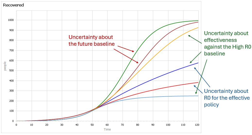
Beyond time 50, there’s a LOT of uncertainty in the disease trajectory, both from the uncontrolled baseline (is R0 low or high?) and the policy effectiveness (do masks work?). The yellow curve (high R0, low effectiveness) illustrates a key feature of epidemics: a policy that falls short of lowering the reproduction ratio below 1 results in continued growth of infection. It’s still beneficial, but constituents are likely to perceive this as a failure and abandon the policy (returning to the baseline, which is worse).
Some of these features are easier to see by looking at the cumulative outcome. Notice that the point prediction for times after about 60 has extremely large variance. But not everything is uncertain. In the uncontrolled baseline runs (green and brownish), eventually almost everyone gets the disease, it’s a matter of when not if, so uncertainty actually decreases after time 90 or so. Also, even though the absolute outcome varies a lot, the policy always improves on the baseline (at least neglecting cost, as we are here). So, while the forecast for time 100 might be bad, the contingent prediction for the effect of the policy is qualitatively insensitive to the uncertainty.
Along with unwise simplification, we also see system dynamics being drawn into attempting what the client wants even when that is unwise or impossible. Of particular note are two kinds of effort—using system dynamics for forecasting, and placing emphasis on a model’s ability to exactly fit historical data.
With regard to forecasting specific future conditions, we face the same barrier that has long plagued econometrics.
Aside from what Forrester is about to discuss, I think there’s also a key difference, as of the time this was written. Econometric models typically employed lots of data and fast computation, but suffered from severe restrictions on functional form (linearity or log-linearity, Normality of distributions, etc.). SD models had essentially unrestricted functional form, particularly with respect to integration and arbitrary nonlinearity, but suffered from insufficient computational power to do everything we would have liked. To some extent, the fields are converging due to loosening of these constraints, in part because the computer under my desk today is now bigger than the fastest supercomputer in the world when I finished my dissertation years ago.
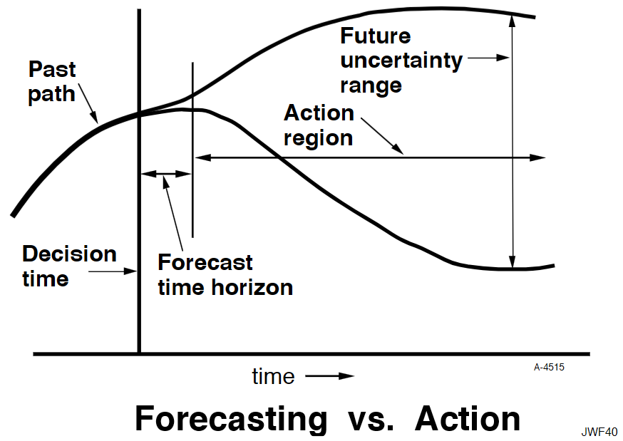
Econometrics has seldom done better in forecasting than would be achieved by naïve extrapolation of past trends. The reasons for that failure also afflict system dynamics. The reasons why forecasting future conditions fail are fundamental in the nature of systems. The following diagram may be somewhat exaggerated, but illustrates my point.
A system variable has a past path leading up to the current decision time. In the short term, the system has continuity and momentum that will keep it from deviating far from an extrapolation of the past. However, random events will cause an expanding future uncertainty range. An effective forecast for conditions at a future time can be made only as far as the forecast time horizon, during which past continuity still prevails. Beyond that horizon, uncertainty is increasingly dominant. However, the forecast is of little value in that short forecast time horizon because a responding decision will be defeated by the very continuity that made the forecast possible. The resulting decision will have its effect only out in the action region when it has had time to pressure the system away from its past trajectory. In other words, one can forecast future conditions in the region where action is not effective, and one can have influence in the region where forecasting is not reliable. You will recall a more complete discussion of this in Appendix K of Industrial Dynamics.
I think Forrester is basically right. However, I think there’s a key qualification. Some things – particularly physical systems – can be forecast quite well, not just because momentum permits extrapolation, but because there is a good understanding of the system. There’s a continuum of forecast skill, between “all models are wrong” and “some models are useful,” and you need to know where you are on that.
Fortunately, your model can tell you about the prospects for forecasting. You can characterize the uncertainty in the model parameters and environmental drivers, generate a distribution of outcomes, and use that to understand where forecasts will begin to fall apart. This is extremely valuable knowledge, and it may be key for implementation. Stakeholders want to know what your intervention is going to do to the system, and if you can’t tell them – with confidence bounds of some sort – they may have no reason to believe your subsequent attributions of success or failure.
In the hallways of SD, I sometimes hear people misconstrue Forrester, to say that “SD doesn’t predict.” This is balderdash. SD is all about prediction. We may not make point predictions of the future state of a system, but we absolutely make predictions about the effects of a policy change, contingent on uncertainties about parameters, structure and external disturbances. If we didn’t do that, what would be the point of the exercise? That’s precisely what JWF is getting at here:
The emphasis on forecasting future events diverts attention from the kind of forecast that system dynamics can reliably make, that is, the forecasting of the kind of continuing effect that an enduring policy change might cause in the behavior of the system. We should not be advising people on the decision they should now make, but rather on how to change policies that will guide future decisions. A properly designed system dynamics model is effective in forecasting how different decision-making policies lead to different kinds of system behavior.