
The incandescent ban is underway.
Conservative think tanks still hate it:
Actually, I think it’s kind of a dumb idea too – but not as bad as you might think, and in the absence of real energy or climate policy, not as dumb as doing nothing. You’d have to be really dumb to believe this:
The ban was pushed by light bulb makers eager to up-sell customers on longer-lasting and much more expensive halogen, compact fluourescent, and LED lighting.
More expensive? Only in a universe where energy and labor costs don’t count (Texas?) and for a few applications (very low usage, or chicken warming).
 Over the last couple years I’ve replaced almost all lighting in my house with LEDs. The light is better, the emissions are lower, and I have yet to see a failure (unlike cheap CFLs).
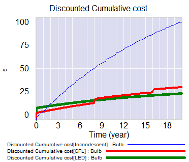
I built a little bulb calculator in Vensim, which shows huge advantages for LEDs in most situations, even with conservative assumptions (low social price of carbon, minimum wage) it’s hard to make incandescents look good. It’s also a nice example of using Vensim for spreadsheet replacement, on a problem that’s not very dynamic but has natural array structure.
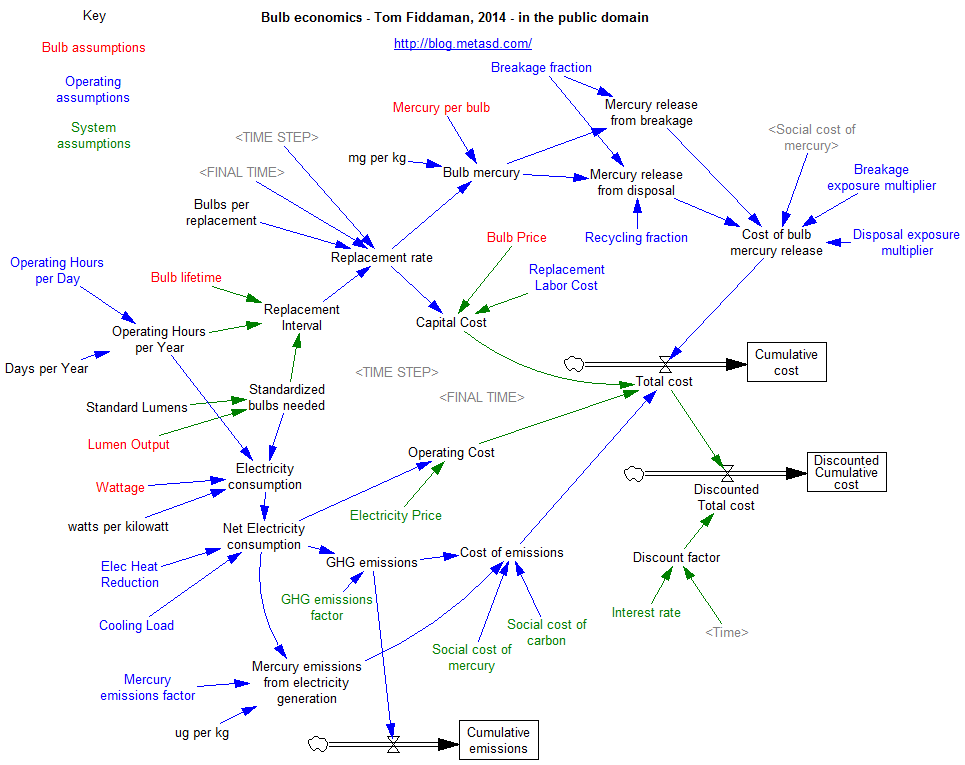 Get it: bulb.mdl or bulb.vpm (uses arrays, so you’ll need the free Model Reader)


