Modeling Investigations

538 had this cool visualization of the Russia investigation in the context of Watergate, Whitewater, and other historic investigations.

The original is fun to watch, but I found it hard to understand the time dynamics from the animation. For its maturity (660 days and counting), has the Russia investigation yielded more or fewer indictments than Watergate (1492 days total)? Are the indictments petering out, or accelerating?

A simplified version of the problem looks a lot like an infection model (a.k.a. logistic growth or Bass diffusion):

So, the interesting question is whether we can – from partway through the history of the system – estimate the ultimate number of indictments and convictions it will yield. This is fraught with danger, especially when you have no independent information about the “physics” of the system, especially the population of potential crooks to be caught. Continue reading “Modeling Investigations”

Polynomials & Interpolating Functions for Decision Rules

Sometimes it’s useful to have a way to express a variable as a flexible function of time, so that you can find the trajectory that maximizes some quantity like profit or fit to data. A caveat: this is not generally the best thing to do. A simple feedback rule will be more robust to rescaling and uncertainty and more informative than a function of time. However, there are times when it’s useful for testing or data approximation to have an open-loop decision rule. The attached models illustrate some options.

If you have access to arrays in Vensim, the simplest is to use the VECTOR LOOKUP function, which reads a subscripted table of values with interpolation. However, that has two limitations: a uniform time axis, and linear interpolation.

If you want a smooth function, a natural option is to pick a polynomial, like

y = a + b*t + c*t^2 + d*t^3 …

However, it can be a little fiddly to interpret the coefficients or get them to produce a desired behavior. The Legendre polynomials provide a basis with nicer scaling, which still recovers the basic linear, quadratic, cubic (etc.) terms when needed. (In terms of my last post, their improved properties make them less sloppy.)


You can generalize these to 2 dimensions by taking tensor products of the 1D series. Another option is to pick the first n terms of Pascal’s triangle. These yield essentially the same result, and either way, things get complex fast.

Back to 1D series, what if you want to express the values as a sequence of x-y points, with smooth interpolation, rather than arcane coefficients? One option is the Lagrange interpolating polynomial. It’s simple to implement, and has continuous derivatives, but it’s an N^2 problem and therefore potentially compute-intensive. It might also behave badly outside its interval, or inside due to ringing.

Probably the best choice for a smooth trajectory specified by x-y points (and optionally, the slope at each point) is a cubic spline or Bezier curve.

Polynomials1.mdl – simple smooth functions, Legendre, Lagrange and spline, runs in any version of Vensim

InterpolatingArrays.mdl InterpolatingArrays.vpm – array functions, VECTOR LOOKUP, Lagrange and spline, requires Pro/DSS or the free Reader

Nelson Rules

I ran across the Nelson Rules in a machine learning package. These are a set of heuristics for detecting changes in statistical process control. Their inclusion felt a bit like navigating a 787 with a mechanical flight computer (which is a very cool device, by the way).

The idea is pretty simple. You have a time series of measurements, normalized to Z-scores, and therefore varying (most of the time) by plus or minus 3 standard deviations. The Nelson Rules provide a way to detect anomalies: drift, oscillation, high or low variance, etc. Rule 1, for example, is just a threshold for outlier detection: it fires whenever a measurement is more than 3 SD from the mean.

In the machine learning context, it seems strange to me to use these heuristics when more powerful tests are available. This is not unlike the problem of deciding whether a random number generator is really random. It’s fairly easy to determine whether it’s producing a uniform distribution of values, but what about cycles or other long-term patterns? I spent a lot of time working on this when we replaced the RNG in Vensim. Many standard tests are available. They’re not all directly applicable, but the thinking is.

In any case, I got curious how the Nelson rules performed in the real world, so I developed a test model.

This feeds a test input (Normally distributed random values, with an optional signal superimposed) into a set of accounting variables that track metrics and compare with the rule thresholds. Some of these are complex.

Rule 4, for example, looks for 14 points with alternating differences. That’s a little tricky to track in Vensim, where we’re normally more interested in continuous time. I tackle that with the following structure:

Difference = Measurement-SMOOTH(Measurement,TIME STEP)
**************************************************************
Is Positive=IF THEN ELSE(Difference>0,1,-1)
**************************************************************
N Switched=INTEG(IF THEN ELSE(Is Positive>0 :AND: N Switched<0
,(1-2*N Switched )/TIME STEP
,IF THEN ELSE(Is Positive<0 :AND: N Switched>0
 ,(-1-2*N Switched)/TIME STEP
 ,(Is Positive-N Switched)/TIME STEP)),0)
**************************************************************
Rule 4=IF THEN ELSE(ABS(N Switched)>14,1,0)
**************************************************************

There’s a trick here. To count alternating differences, we need to know (a) the previous count, and (b) whether the previous difference encountered was positive or negative. Above, N Switched stores both pieces of information in a single stock (INTEG). That’s possible because the count is discrete and positive, so we can overload the storage by giving it the sign of the previous difference encountered.

Thus, if the current difference is negative (Is Positive < 0) and the previous difference was positive (N Switched > 0), we (a) invert the sign of the count by subtracting 2*N Switched, and (b) augment the count, here by subtracting 1 to make it more negative.

Similar tricks are used elsewhere in the structure.

How does it perform? Surprisingly well. Here’s what happens when the measurement distribution shifts by one standard deviation halfway through the simulation:

There are a few false positives in the first 1000 days, but after the shift, there are many more detections from multiple rules.

The rules are pretty good at detecting a variety of pathologies: increases or decreases in variance, shifts in the mean, trends, and oscillations. The rules also have different false positive rates, which might be OK, as long as they catch nonoverlapping problems, and don’t have big differences in sensitivity as well. (The original article may have more to say about this – I haven’t checked.)

However, I’m pretty sure that I could develop some pathological inputs that would sneak past these rules. By contrast, I’m pretty sure I’d have a hard time sneaking anything past the NIST or Diehard RNG test suites.

If I were designing this from scratch, I’d use machine learning tools more directly – there are lots of tests for distributions, changes, trend breaks, oscillation, etc. that can be used online with a consistent likelihood interpretation and optimal false positive/negative tradeoffs.

Here’s the model:

NelsonRules1.mdl

NelsonRules1.vpm

The Ambiguity of Causal Loop Diagrams and Archetypes

I find causal loop diagramming to be a very useful brainstorming and presentation tool, but it falls short of what a model can do for you.

Here’s why. Consider the following pair of archetypes (Eroding Goals and Escalation, from wikipedia):

Eroding Goals and Escalation archetypes

Archetypes are generic causal loop diagram (CLD) templates, with a particular behavior story. The Escalation and Eroding Goals archetypes have identical feedback loop structures, but very different stories. So, there’s no unique mapping from feedback loops to behavior. In order to predict what a set of loops is going to do, you need more information.

Here’s an implementation of Eroding Goals:

Notice several things:

  • I had to specify where the stocks and flows are.
  • “Actions to Improve Goals” and “Pressure to Adjust Conditions” aren’t well defined (I made them proportional to “Gap”).
  • Gap is not a very good variable name.
  • The real world may have structure that’s not mentioned in the archetype (indicated in red).

Here’s Escalation:

The loop structure is mathematically identical; only the parameterization is different. Again, the missing information turns out to be crucial. For example, if A and B start with the same results, there is no escalation – A and B results remain constant. To get escalation, you either need (1) A and B to start in different states, or (2) some kind of drift or self-excitation in decision making (green arrow above).

Even then, you may get different results. (2) gives exponential growth, which is the standard story for escalation. (1) gives escalation that saturates:

The Escalation archetype would be better if it distinguished explicit goals for A and B results. Then you could mathematically express the key feature of (2) that gives rise to arms races:

  • A’s goal is x% more bombs than B
  • B’s goal is y% more bombs than A

Both of these models are instances of a generic second-order linear model that encompasses all possible things a linear model can do:

Notice that the first-order and second-order loops are disentangled here, which makes it easy to see the “inner” first order loops (which often contribute damping) and the “outer” second order loop, which can give rise to oscillation (as above) or the growth in the escalation archetype. That loop is difficult to discern when it’s presented as a figure-8.

Of course, one could map these archetypes to other figure-8 structures, like:

How could you tell the difference? You probably can’t, unless you consider what the stocks and flows are in an operational implementation of the archetype.

The bottom line is that the causal loop diagram of an archetype or anything else doesn’t tell you enough to simulate the behavior of the system. You have to specify additional assumptions. If the system is nonlinear or stochastic, there might be more assumptions than I’ve shown above, and they might be important in new ways. The process of surfacing and testing those assumptions by building a stock-flow model is very revealing.

If you don’t build a model, you’re in the awkward position of intuiting behavior from structure that doesn’t uniquely specify any particular mode. In doing so, you might be way ahead of non-systems thinkers approaching the same problem with a laundry list. But your ability to discover errors, incorporate data and discover leverage is far greater if you can simulate.

The model: wikiArchetypes1b.mdl (runs in any version of Vensim)

Dynamics of the last Twinkie

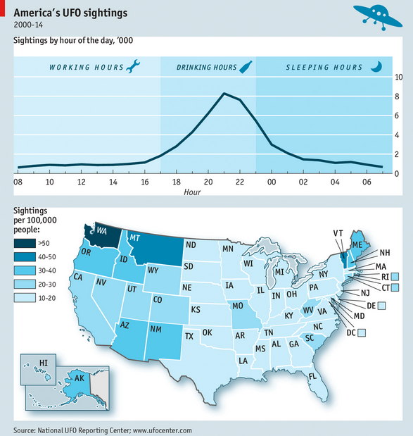
When Hostess went bankrupt in 2012, there was lots of speculation about the fate of the last Twinkie, perhaps languishing on the dusty shelves of a gas station convenience store somewhere in New Mexico. Would that take ten days, ten weeks, ten years?

So, what does this have to do with system dynamics? It calls to mind the problem of modeling the inventory stockout constraint on sales. This problem dates back to Industrial Dynamics (see the variable NIR driving SSR and the discussion around figs. 15-5 and 15-7).

If there’s just one product in one inventory (i.e. one store), and visibility doesn’t matter, the constraint is pretty simple. As long as there’s one item left, sales or shipments can proceed. The constraint then is:

(1) selling = MIN(desired selling, inventory/time step)

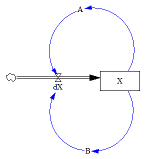
In other words, the most that can be sold in one time step is the amount of inventory that’s actually on hand. Generically, the constraint looks like this:

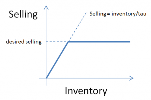
Here, tau is a time constant, that could be equal to time step (DT), as above, or could be generalized to some longer interval reflecting handling and other lags.

This can be further generalized to some kind of continuous function, like:

(2) selling = desired selling * f( inventory )

where f() is often a lookup table. This can be a bit tricky, because you have to ensure that f() goes to zero fast enough to obey the inventory/DT constraint above.

But what if you have lots of products and/or lots of inventory points, perhaps with different normal turnover rates? How does this aggregate? I built the following toy model to find out. You could easily do this in Vensim with arrays, but I found that it was ideally suited to Ventity.
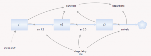
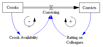
Here’s the setup:

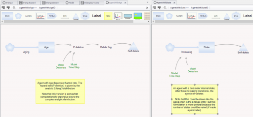
First, there’s a collection of Store entities, each with an inventory. Initial inventory is random, with a Poisson distribution, which ensures integer twinkies. Customer arrivals also have a Poisson distribution, and (optionally), the mean arrival rate varies by store. Selling is constrained to stock on hand via inventory/DT, and is also subject to a visibility effect – shelf stock influences the probability that a customer will buy a twinkie (realized with a Binomial distribution). The visibility effect saturates, so that there are diminishing returns to adding stock, as occurs when new stock goes to the back rows of the shelf, for example.

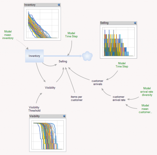
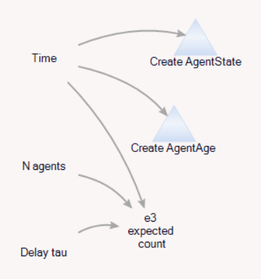
In addition, there’s an Aggregate entitytype, which is very similar to the Store, but deterministic and continuous.

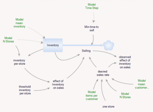
The Aggregate’s initial inventory and sales rates are set to the expected values for individual stores. Two different kinds of constraints on the inventory outflow are available: inventory/tau, and f(inventory). The sales rate simplifies to:

(3) selling = min(desired sales rate*f(inventory),Inventory/Min time to sell)

(4) min time to sell >= time step

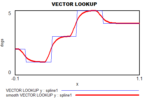
In the Store and the Aggregate, the nonlinear effect of inventory on sales (called visibility in the store) is given by

(5) f(inventory) = 1-Exp(-Inventory/Threshold)

However, the aggregate threshold might be different from the individual store threshold (and there’s no compelling reason for the aggregate f() to match the individual f(); it was just a simple way to start).

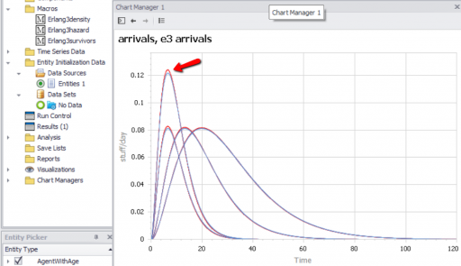
In the Store[] collection, I calculate aggregates of the individual stores, which look quite continuous, even though the population is only 100. (There are over 100,000 gas stations in the US.)

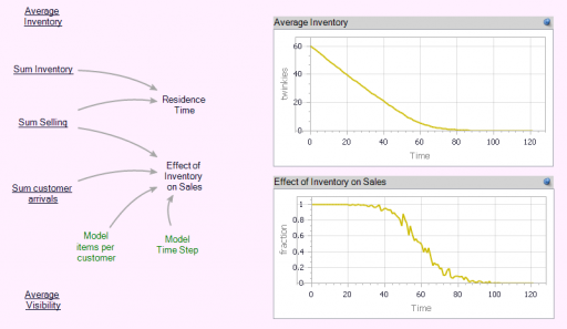
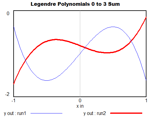
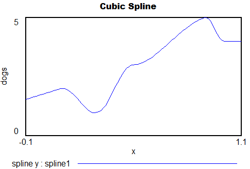
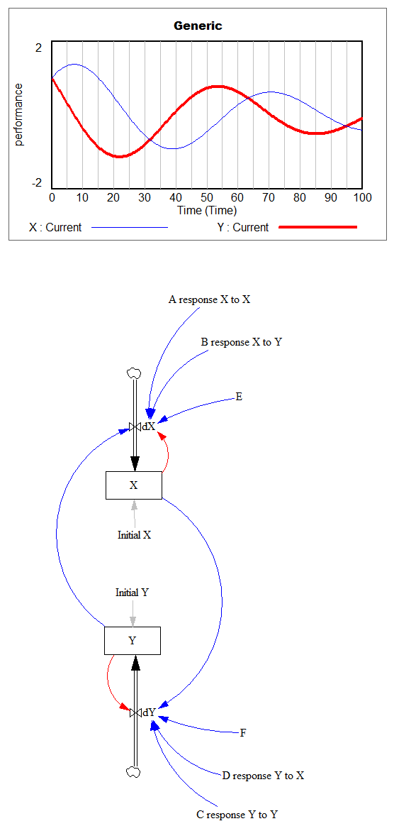
Notice that the time series behavior of the effect of inventory on sales is sigmoid.

Now we can compare individual and aggregate behavior:
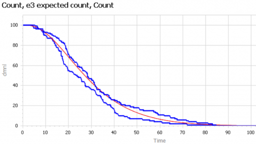
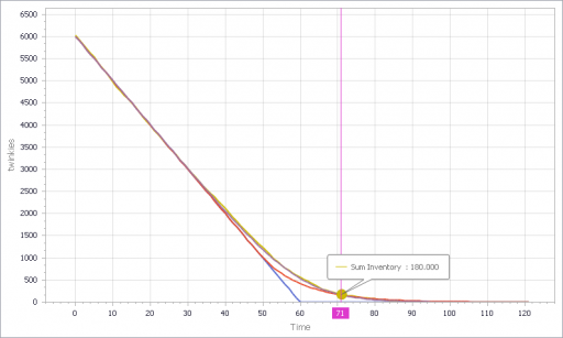
Inventory

Selling

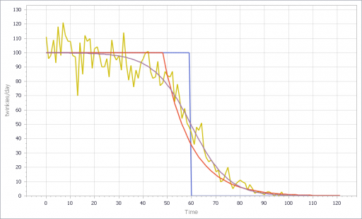
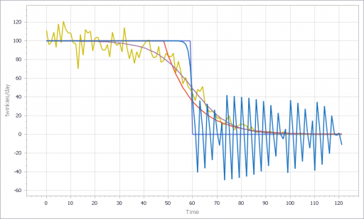
The noisy yellow line is the sum of the individual Stores. The blue line arises from imposing a hard cutoff, equation (1) above. This is like assuming that all stores are equal, and inventory doesn’t affect sales, until it’s gone. Clearly it’s not a great fit, though it might be an adequate shortcut where inventory dynamics are not really the focus of a model.

The red line also imposes an inventory/tau constraint, but the time constant (tau) is much longer than the time step, at 8 days (time step = 1 day). Finally, the purple sigmoid line arises from imposing the nonlinear f(inventory) constraint. It’s quite a good fit, but the threshold for the aggregate must be about twice as big as for the individual Stores.

However, if you parameterize f() poorly, and omit the inventory/tau constraint, you get what appear to be chaotic oscillations – cool, but obviously unphysical:

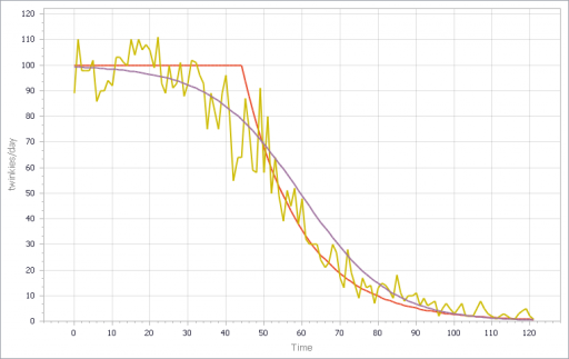
If, in addition, you add diversity in Store’s customer arrival rates, you get a longer tail on inventory. That last Twinkie is likely to be in a low-traffic outlet. This makes it a little tougher to fit all parts of the curve:

I think there are some interesting questions here, that would make a great paper for the SD conference:

  • (Under what conditions) can you derive the functional form of the aggregate constraint from the properties of the individual Stores?
  • When do the deficiencies of shortcut approaches, that may lack smooth derivatives, matter in aggregate models like Industrial dynamics?
  • What are the practical implications for marketing models?
  • What can you infer about inventory levels from aggregate data alone?
  • Is that really chaos?

Have at it!

The Ventity model: LastTwinkie1.zip

Job tenure dynamics

This is a simple model of the dynamics of employment in a sector. I built it for a LinkedIn article that describes the situation and the data.

The model is interesting and reasonably robust, but it has (at least) three issues you should know about:

  • The initialization in equilibrium isn’t quite perfect.
  • The sector-entry decision (Net Entering) is not robust to low unemployment. In some situations, a negative net entering flow could cause negative Job Seekers.
  • The sector-entry decision also formulates attractiveness exclusively as a function of salaries; in fact, it should also account for job availability (perceived vacancy and unemployment rates).

Correcting these shortcomings shouldn’t be too hard, and it should make the model’s oscillatory tendencies more realistic. I leave this as an exercise for you. Drop me a note if you have an improved version.

The model requires Vensim (any version, including free PLE).

Download employees1.mdl

Forrester on Continuous Flows

I just published three short videos with sample models, illustrating representation of discrete and random events in Vensim.

Jay Forrester‘s advice from Industrial Dynamics is still highly relevant. Here’s an excerpt:

Chapter 5, Principles for Formulating Models

5.5 Continuous Flows

In formulating a model of an industrial operation, we suggest that the system be treated, at least initially, on the basis of continuous flows and interactions of the variables. Discreteness of events is entirely compatible with the concept of information-feedback systems, but we must be on guard against unnecessarily cluttering our formulation with the detail of discrete events that only obscure the momentum and continuity exhibited by our industrial systems.

In beginning, decisions should be formulated in the model as if they were continuously (but not implying instantaneously) responsive to the factors on which they are based. This means that decisions will not be formulated for intermittent reconsideration each week, month or year. For example, factory production capacity would vary continuously, not by discrete additions. Ordering would go on continuously, not monthly when the stock records are reviewed.

There are several reasons for recommending the initial formulation of a continuous model:

  • Real systems are more nearly continuous than is commonly supposed …
  • There will usually be considerable “aggregation” …
  • A continuous-flow system is usually an effective first approximation …
  • There is a natural tendency of model builders and executives to overstress the discontinuities of real situations. …
  • A continuous-flow model helps to concentrate attention on the central framework of the system. …
  • As a starting point, the dynamics of the continuous-flow model are usually easier to understand …
  • A discontinuous model, which is evaluated at infrequent intervals, such as an economic model solved for a new set of values annually, should never be justified by the fact that data in the real system have been collected at such infrequent intervals. …

These comments should never be construed as suggesting that the model builder should lack interest in the microscopic separate events that occur in a continuous-flow channel. The course of the continuous flow is the course of the separate events in it. By studying individual events we get a picture of how decisions are made and how the flows are delayed. The study of individual events is on of our richest sources of information about the way the flow channels of the model should be constructed. When a decision is actually being made regularly on a periodic basis, like once a month, the continuous-flow equivalent channel should contain a delay of half the interval; this represents the average delay encountered by information in the channel.

The preceding comments do not imply that discreteness is difficult to represent, nor that it should forever be excluded from a model. At times it will become significant. For example, it may create a disturbance that will cause system fluctuations that can be mistakenly interreted as externally generated cycles (…). When a model has progressed to the point where such refinements are justified, and there is reason to believe that discreteness has a significant influence on system behavior, discontinuous variables should then be explored to determine their effect on the model.

[Ellipses added – see the original for elaboration.]

Dynamics of Term Limits

I am a little encouraged to see that the very top item on Trump’s first 100 day todo list is term limits:

* FIRST, propose a Constitutional Amendment to impose term limits on all members of Congress;

Certainly the defects in our electoral and campaign finance system are among the most urgent issues we face.

Assuming other Republicans could be brought on board (which sounds unlikely), would term limits help? I didn’t have a good feel for the implications, so I built a model to clarify my thinking.

I used our new tool, Ventity, because I thought I might want to extend this to multiple voting districts, and because it makes it easy to run several scenarios with one click.

Here’s the setup:

structure

The model runs over a long series of 4000 election cycles. I could just as easily run 40 experiments of 100 cycles or some other combination that yielded a similar sample size, because the behavior is ergodic on any time scale that’s substantially longer than the maximum number of terms typically served.

Each election pits two politicians against one another. Normally, an incumbent faces a challenger. But if the incumbent is term-limited, two challengers face each other.

The electorate assesses the opponents and picks a winner. For challengers, there are two components to voters’ assessment of attractiveness:

  • Intrinsic performance: how well the politician will actually represent voter interests. (This is a tricky concept, because voters may want things that aren’t really in their own best interest.) The model generates challengers with random intrinsic attractiveness, with a standard deviation of 10%.
  • Noise: random disturbances that confuse voter perceptions of true performance, also with a standard deviation of 10% (i.e. it’s hard to tell who’s really good).

Once elected, incumbents have some additional features:

  • The assessment of attractiveness is influenced by an additional term, representing incumbents’ advantages in electability that arise from things that have no intrinsic benefit to voters. For example, incumbents can more easily attract funding and press.
  • Incumbent intrinsic attractiveness can drift. The drift has a random component (i.e. a random walk), with a standard deviation of 5% per term, reflecting changing demographics, technology, etc. There’s also a deterministic drift, which can either be positive (politicians learn to perform better with experience) or negative (power corrupts, or politicians lose touch with voters), defaulting to zero.
  • The random variation influencing voter perceptions is smaller (5%) because it’s easier to observe what incumbents actually do.

There’s always a term limit of some duration active, reflecting life expectancy, but the term limit can be made much shorter.

Here’s how it behaves with a 5-term limit:

terms

Politicians frequently serve out their 5-term limit, but occasionally are ousted early. Over that period, their intrinsic performance varies a lot:

attractiveness

Since the mean challenger has 0 intrinsic attractiveness, politicians outperform the average frequently, but far from universally. Underperforming politicians are often reelected.

Over a long time horizon (or similarly, many districts), you can see how average performance varies with term limits:

long

With no learning, as above, term limits degrade performance a lot (top panel). With a 2-term limit, the margin above random selection is about 6%, whereas it’s twice as great (>12%) with a 10-term limit. This is interesting, because it means that the retention of high-performing politicians improves performance a lot, even if politicians learn nothing from experience.

This advantage holds (but shrinks) even if you double the perception noise in the selection process. So, what does it take to justify term limits? In my experiments so far, politician performance has to degrade with experience (negative learning, corruption or losing touch). Breakeven (2-term limits perform the same as 10-term limits) occurs at -3% to -4% performance change per term.

But in such cases, it’s not really the term limits that are doing the work. When politician performance degrades rapidly with time, voters throw them out. Noise may delay the inevitable, but in my scenario, the average politician serves only 3 terms out of a limit of 10. Reducing the term limit to 1 or 2 does relatively little to change performance.

Upon reflection, I think the model is missing a key feature: winner-takes-all, redistricting and party rules that create safe havens for incompetent incumbents. In a district that’s split 50-50 between brown and yellow, an incompetent brown is easily displaced by a yellow challenger (or vice versa). But if the split is lopsided, it would be rare for a competent yellow challenger to emerge to replace the incompetent yellow incumbent. In such cases, term limits would help somewhat.

I can simulate this by making the advantage of incumbency bigger (raising the saturation advantage parameter):

attractiveness2

However, long terms are a symptom of the problem, not the root cause. Therefore it probably necessary in addition to address redistricting, campaign finance, voter participation and education, and other aspects of the electoral process that give rise to the problem in the first place. I’d argue that this is the single greatest contribution Trump could make.

You can play with the model yourself using the Ventity beta/trial and this model archive:

termlimits4.zip

The dynamics of UFO sightings

The Economist reports on UFO sightings:

UFOdataThis deserves a model:

UFOs

UFOs.vpm (Vensim published model, requires Pro/DSS or the free Reader)

The model is a mixed discrete/continuous simulation of an individual sleeping, working and drinking. This started out as a multi-agent model, but I realized along the way that sleeping, working and drinking is a fairly ergodic process on long time scales (at least with respect to UFOs), so one individual with a distribution of behaviors over time or simulations is as good as a population of agents.

The model replicates the data somewhat faithfully:

UFOdistributionThe model shows a morning peak (people awake but out and about) and a workday dip (inside, lurking near the water cooler) but the data do not. This suggests to me that:

  • Alcohol is the dominant factor in sightings.
  • I don’t party nearly enough to see a UFO.

Actually, now that I’ve built this version, I think the interesting model would have a longer time horizon, to address the non-ergodic part: contagion of sightings across individuals.

h/t Andreas Größler.

Bulbs banned

The incandescent ban is underway.

Conservative think tanks still hate it:

Actually, I think it’s kind of a dumb idea too – but not as bad as you might think, and in the absence of real energy or climate policy, not as dumb as doing nothing. You’d have to be really dumb to believe this:

The ban was pushed by light bulb makers eager to up-sell customers on longer-lasting and much more expensive halogen, compact fluourescent, and LED lighting.

More expensive? Only in a universe where energy and labor costs don’t count (Texas?) and for a few applications (very low usage, or chicken warming).

bulb economicsOver the last couple years I’ve replaced almost all lighting in my house with LEDs. The light is better, the emissions are lower, and I have yet to see a failure (unlike cheap CFLs).

I built a little bulb calculator in Vensim, which shows huge advantages for LEDs in most situations, even with conservative assumptions (low social price of carbon, minimum wage) it’s hard to make incandescents look good. It’s also a nice example of using Vensim for spreadsheet replacement, on a problem that’s not very dynamic but has natural array structure.

bulbModelGet it: bulb.mdl or bulb.vpm (uses arrays, so you’ll need the free Model Reader)