Don't just do something, stand there! Reflections on the counterintuitive behavior of complex systems, seen through the eyes of System Dynamics, Systems Thinking and simulation.
This video explores a simple epidemic model for a community confronting coronavirus.
I built this to reflect my hometown, Bozeman MT and surrounding Gallatin County, with a population of 100,000 and no reported cases – yet. It shows the importance of an early, robust, multi-pronged approach to reducing infections. Because it’s simple, it can easily be adapted for other locations.
Why border control has limits, and mild cases don’t matter.
At the top, the US coronavirus response seems to be operating with (at least) two misperceptions. First, that border control works. Second, that a lower fatality rate means fewer deaths. Here’s how it really works.
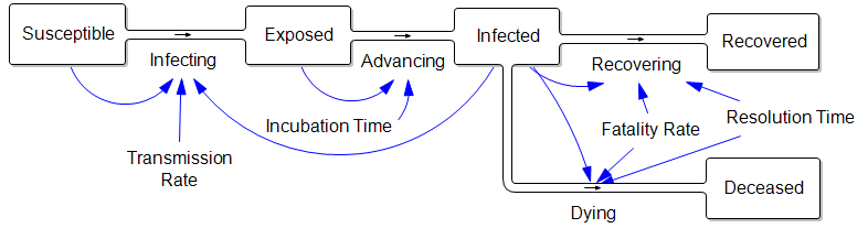
Consider an extremely simplified SEIRD model. This is a generalization of the simple SIR framework to include asymptomatic, non-infective Exposed people and the Deceased:
The parameters are such that the disease takes about a week to incubate, and about a week to resolve. The transmission rate is such that cases double about once a week, if left uncontrolled.
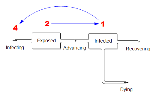
Those fortuitous time constants make it really simple to model the spread in discrete time. First, abstract away the susceptible (who are abundant early in the epidemic) and the resolved cases (which are few and don’t participate further):
In this dirt-simple model,
This week’s infected will all resolve
This week’s exposed will advance to become next week’s infected
Next week’s exposed are the ones the current infected are infecting now.
If the disease is doubling weekly, then for every 1 infected person there must be 2 exposed people in the pipeline. And each of those infected people must expose 4 others. (Note that this is seemingly an R0 of 4, which is higher than what’s usually quoted, but the difference is partly due to discrete vs. continuous compounding. The R0 of 2.2 that’s currently common seems too low to fit the data though – more on that another time.)
What does this imply for control strategy? It means that, on the day you close the border, the infected arrivals you’ve captured and isolated understate the true problem. For every infected person, there are two exposed people on the loose, initiating domestic community spread. Because it’s doubling weekly, community infections very quickly replace the imports, even if a travel ban is 100% effective.
Mild Cases
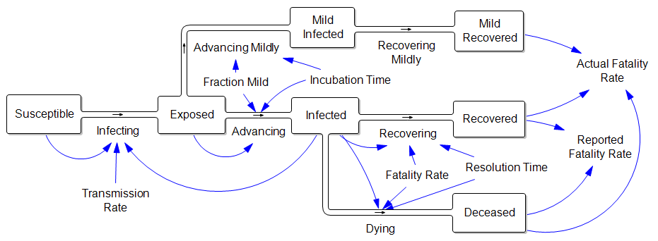
Now consider the claim that the fatality rate is much lower than reported, because there are many unobserved mild cases:
In other words, the reported fatality rate is Deceased/(Recovered+Deceased), but the “real” fatality rate is Deceased/(Recovered+Deceased+Mild Recovered). That’s great, but where did all those mild cases come from? If they are sufficiently numerous to dilute the fatality rate by, say, a factor of 10, then there must also be 9 people with mild infections going undetected for every known infected case. That doesn’t help the prognosis for deaths a bit, because (one tenth the fatality rate) x (ten times the cases) yields the same outcome. Actually, this makes the border control and community containment problem much harder, because there are now 10x as many contacts to trace and isolate. Fortunately this appears to be pure speculation.
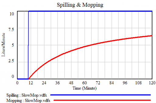
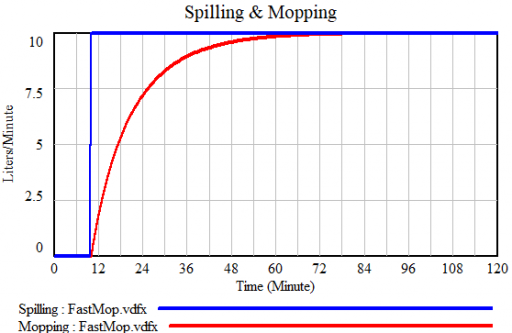
I just learned a beautiful Dutch idiom, dweilen met de kraan open. It means “mopping [the floor] with the the faucet running.” I’m not sure there’s a common English equivalent that’s so poetic, but perhaps “treating the symptoms, not the cause” is closest.
This makes a nice little model:
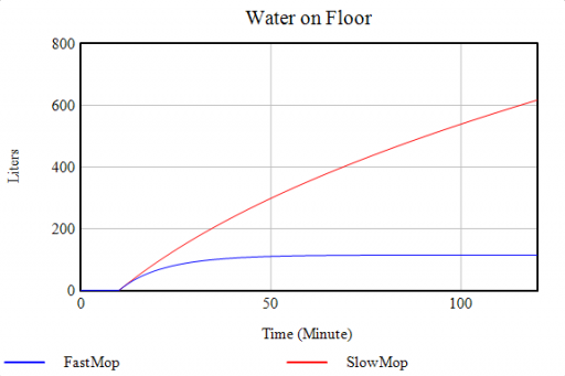
If you’re a slow mopper, you can never catch up with the tap:
If you’re fast, you can catch up, but not reverse the process:
Either way, as long as you don’t turn off the tap, there will always be water on the floor:
The structure of the system above is nearly the same as filling a leaky bucket, except that the user is concerned with the inflow rather than the outflow.
Beating a dead horse and fiddling while Rome burns
These control systems are definitely going nowhere:
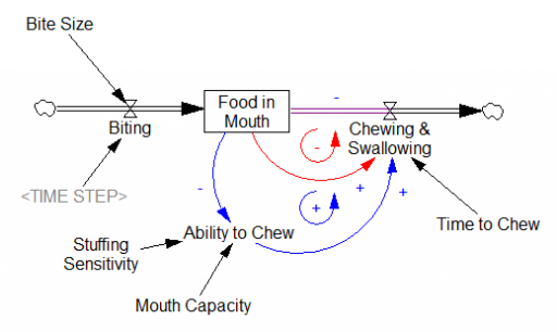
Biting off more than you can chew
This one’s fun because it only becomes an exercise in futility when you cross a nonlinear threshold.
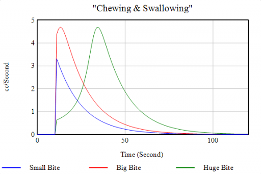
As long as you take small bites, the red loop of “normal” chewing clears the backlog of food in mouth in a reasonable time. But when you take a huge bite, you exceed the mouth’s capacity. This activates the blue positive loop, which slows chewing until the burden has been reduced somewhat. When the blue loop kicks in, the behavior mode changes (green), greatly delaying the process:
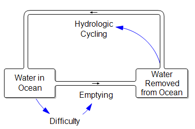
I think the futility of this endeavor is normally thought of as a question of scale. The volume of the ocean is about 1.35 trillion trillion cubic centimeters, and a thimble contains about 1 cc. But suppose you could cycle that thimble really fast? I think you still have feedback problems:
First, you have the mopping problem: as the ocean empties, the job gets harder, because you’ll be carrying water uphill … a lot (the average depth of the ocean is about 4000 meters). Second, you have the leaky bucket problem. Where are you going to put all that water? Evaporation and surface flow are inevitably going to take some back to the ocean.
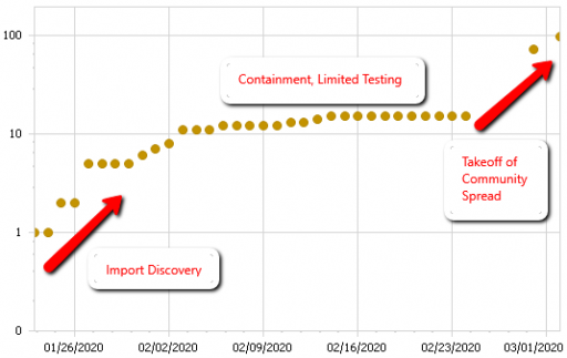
I ran across this twitter thread this morning, describing how a focus on border security and containment of existing cases has failed to prevent the takeoff of coronavirus.
Here’s the data on US confirmed cases that goes with it:
US confirmed coronavirus cases, as of 3/2/2019. Source: Johns Hopkins CSSE dashboard, https://gisanddata.maps.arcgis.com/apps/opsdashboard/index.html#/bda7594740fd40299423467b48e9ecf6
It’s easy to see how this behavior could lure managers into a self-confirming attributions trap. After a surge of imports, they close the borders. Cases flatten. Problem solved. Why go looking for trouble?
The problem is that containment alone doesn’t work, because the structure of the system defeats it. You can’t intercept every infected person, because some are exposed but not yet symptomatic, or have mild cases. As soon as a few of these people slip into the wild, the positive loops that drive infection operate as they always have. Once the virus is in the wild, it’s essential to change behavior enough to lower its reproduction below replacement.
Markets collapse when they’re in a vulnerable state. Coronavirus might be the straw that broke the camel’s back – this time – but there’s no clear pandemic to stock price causality.
The predominant explanation for this week’s steep decline in the stock market is coronavirus. I take this as evidence that the pandemic of open-loop, event-based thinking is as strong as ever.
First, let’s look at some data. Here’s interest in coronavirus:
It was already pretty high at the end of January. Why didn’t the market collapse then? (In fact, it rose a little over February). Is there a magic threshold of disease, beyond which markets collapse?
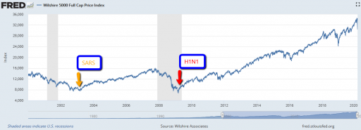
How about other pandemics? Interest in pandemics was apparently higher in 2009, with the H1N1 outbreak:
Did the market collapse then? No. In fact, that was the start of the long climb out of the 2007 financial crisis. The same was true for SARS, in spring 2003, in the aftermath of the dotcom bust.
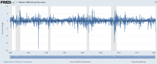
There are also lots of examples of market crashes, like 1987, that aren’t associated with pandemic fears at all. Corrections of this magnitude are actually fairly common (especially if you consider the percentage drop, not the inflated absolute drop):
Wilshire Associates, Wilshire 5000 Full Cap Price Index [WILL5000PRFC], retrieved from FRED, Federal Reserve Bank of St. Louis; https://fred.stlouisfed.org/series/WILL5000PRFC, February 28, 2020.So clearly a pandemic is neither necessary nor sufficient for a market correction to occur.
I submit that the current attribution of the decline to coronavirus is primarily superstitious, and that the market is doing what it always does.
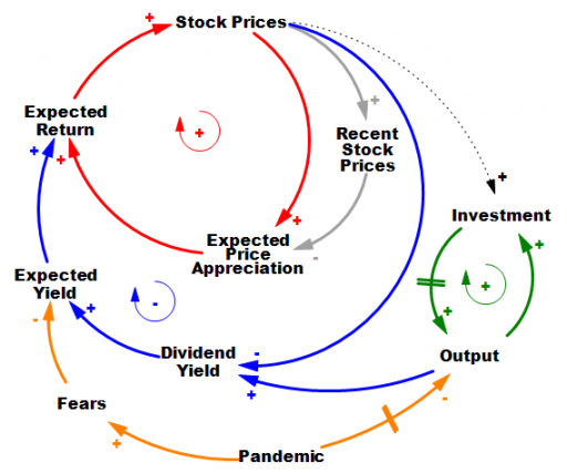
It’s hard to do it justice briefly, but the stock market is basically an overlay of a complicated allocation mechanism on top of the real economy. In the real economy (green positive loop) capital and technology accumulation increase output (thinking strictly of on-market effects). Growth in that loop proceeds steadily in the long run, but with bumps from business cycles. The stock market is sending signals to the real economy about how to invest, but that’s complicated, hence the dashed line.
In the stock market, prices reflect expectations about the future flow of dividends from the economy (blue negative loop). If that were the whole story, coronavirus (orange) would have to have induced fears of a drop in the NPV of future profits of about 10%. Hopefully that’s way outside any plausible scenario. So why the big drop? It’s due to the other half of the story. Expectations are formed partly on fundamentals, and partly on the expectation that the market will go up, because it’s been going up (red positive loop).
There are actually a number of mechanisms behind this: naive extrapolation, sophisticated exploitation of the greater fool, redirection of media attention to prognosticators of growth when they’re right, and so on. The specifics aren’t important; what matters is that they create a destabilizing reinforcing feedback loop that inflates bubbles. Then, when some shock sufficient to overcome the expectations of appreciation arrives, the red loop runs the other way, as a vicious cycle. Diminished expected returns spark selling, lowering prices, and further diminishing expectations of appreciation. If things get bad enough, liquidity problems and feedback to the real economy accentuate the problem, as in 1929.
Importantly, this structure makes the response of the market to bad news nonlinear and state-dependent. When SARS and H1N1 arrived, the market was already bottomed out. At such a point, the red loop is weak, because there’s not much speculative activity or enthusiasm. The fact that this pandemic is having a large impact, even while it’s still hypothetical, suggests that market expectations were already in a fragile state. If SARS-Cov-2 hadn’t come along to pop the bubble, some other sharp object would have done it soon: a bank bust, a crop failure, or maybe just a bad hot dog for an influential trader.
Coronavirus may indeed be the proximate cause of this week’s decline, in the same sense as the straw that broke the camel’s back. However, the magnitude of the decline is indicative of the fragility of the market state when the shock came along, and not necessarily of the magnitude of the shock itself. The root cause of the decline is that the structure of markets is prone to abrupt losses.
I’ve been looking at early model-based projections for the coronavirus outbreak (SARS-CoV-2, COVID-19). The following post collects some things I’ve found informative. I’m eager to hear of new links in the comments.
The original SIR epidemic model, by Kermack and McKendrick. Very interesting to see how they thought about it in the pre-computer era, and how durable their analysis has been:
This blog post by Josh at Cassandra Capital collects quite a bit more interesting literature, and fits a simple SIR model to the data. I can’t vouch for the analysis because I haven’t looked into it in detail, but the links are definitely useful. One thing I note is that his fatality rate (12%) is much higher than in other sources I’ve seen (.5-3%) so hopefully things are less dire than shown here.
I had high hopes that social media might provide early links to breaking literature, but unfortunately the signal is swamped by rumors and conspiracy theories. The problem is made more difficult by naming – coronavirus, COVID19, SARS-CoV-2, etc. If you don’t include “mathematical model” or similar terms in your search, it’s really hopeless.
If your interested in exploring this yourself, the samples in the standard Ventity distribution include a family of infection models. I plan to update some of these and report back.
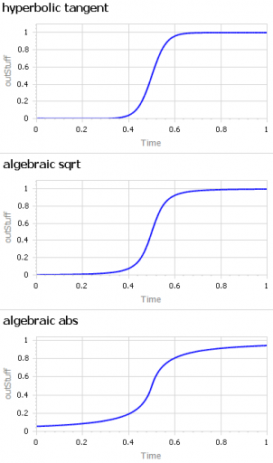
A question about sigmoid functions prompted me to collect a lot of small models that I’ve used over the years.
A sigmoid function is just a function with a characteristic S shape. (OK, you have to use your imagination a bit to get the S.) These tend to arise in two different ways:
As a nonlinear response, where increasing the input initially has little effect, then considerable effect, then saturates with little effect. Neurons, and transfer functions in neural networks, behave this way. Advertising is also thought to work like this: too little, and people don’t notice. Too much, and they become immune. Somewhere in the middle, they’re responsive.
Dynamically, as the behavior over time of a system with shifting dominance from growth to saturation. Examples include populations approaching carrying capacity and the Bass diffusion model.
Correspondingly, there are (at least) two modeling situations that commonly require the use of some kind of sigmoid function:
You want to represent the kind of saturating nonlinear effect described above, with some parameters to control the minimum and maximum values, the slope around the central point, and maybe symmetry features.
You want to create a simple scenario generator for some driver of your model that has logistic behavior, but you don’t want to bother with an explicit dynamic structure.
The examples in this model address both needs. They include:
I’m sure there are still a lot of alternatives I omitted. Cubic splines and Bezier curves come to mind. I’d be interested to hear of any others of interest, or just alternative parameterizations of things already here.
An interesting exploration of the limits of data-driven predictions in nonlinear dynamic problems:
Assessing the predictability of nonlinear dynamics under smooth parameter changes
Simone Cenci, Lucas P. Medeiros, George Sugihara and Serguei Saavedra https://doi.org/10.1098/rsif.2019.0627
Short-term forecasts of nonlinear dynamics are important for risk-assessment studies and to inform sustainable decision-making for physical, biological and financial problems, among others. Generally, the accuracy of short-term forecasts depends upon two main factors: the capacity of learning algorithms to generalize well on unseen data and the intrinsic predictability of the dynamics. While generalization skills of learning algorithms can be assessed with well-established methods, estimating the predictability of the underlying nonlinear generating process from empirical time series remains a big challenge. Here, we show that, in changing environments, the predictability of nonlinear dynamics can be associated with the time-varying stability of the system with respect to smooth changes in model parameters, i.e. its local structural stability. Using synthetic data, we demonstrate that forecasts from locally structurally unstable states in smoothly changing environments can produce significantly large prediction errors, and we provide a systematic methodology to identify these states from data. Finally, we illustrate the practical applicability of our results using an empirical dataset. Overall, this study provides a framework to associate an uncertainty level with short-term forecasts made in smoothly changing environments.


 The problem is that containment alone doesn’t work, because the structure of the system defeats it. You can’t intercept every infected person, because some are exposed but not yet symptomatic, or have mild cases. As soon as a few of these people slip into the wild, the positive loops that drive infection operate as they always have. Once the virus is in the wild, it’s essential to change behavior enough to lower its reproduction below replacement.