Sometimes the best model is the data, but all data are wrong! A big part of validation is detecting and correcting errors in data.
I’ve recently run across an interesting example. I’m working on Chronic Wasting Disease in deer, which essentially combines an epidemiology model with a deer population model, surrounded by some social and environmental features.
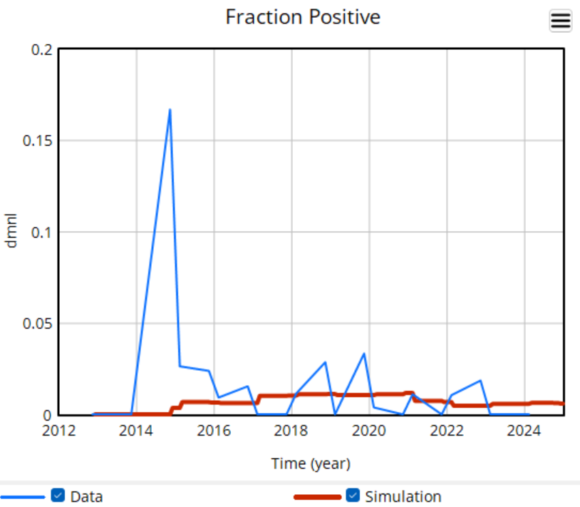
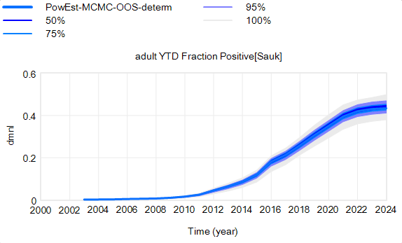
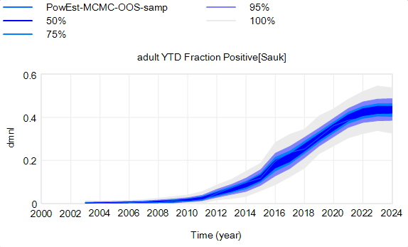
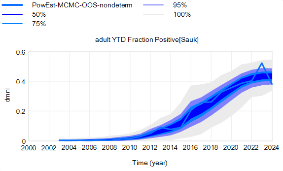
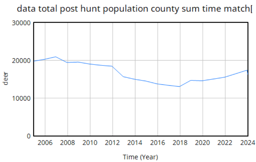
We use data heavily. The model is driven by hunter harvest and targeted removals of deer, which are fairly reliable measurement streams with long histories. We calibrate primarily against surveillance (positive CWD tests) and population data. The surveillance is very noisy because sample sizes are small, but as far as we know it’s fairly free of big systematic problems. The population data is more aggregate and less noisy. It typically looks like this:
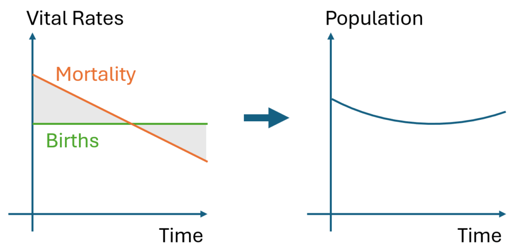
The U-shaped pattern here is intuitively attractive, because it’s doing bathtub dynamics. Population integrates the difference between births and deaths (shaded area, left plot – or really its negative). In reality mortality is declining (due to declining hunting pressure), so a population that declines early, levels off, and later grows is a plausible outcome.
However … it proves difficult to replicate this trajectory with realistic parameters. Part of the problem is that there are two discontinuities:
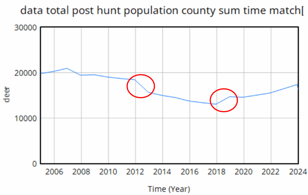
The first one is real – it’s an EHD outbreak that caused widespread mortality. That can easily be captured in the model with an exogenous event. The second one though turns out to be a change in methods, and that’s the real problem here. This deer “data” isn’t really data, it’s an accounting model with its own assumptions. Really there’s no such thing as pure data – it’s always captured through some kind of process that is effectively a model. But in this case, the model is problematic, because it changed in 2018, and we don’t know how.
We do know it’s wrong though. Difficulty tuning a model to the data led us look into the details of the age structure, and it’s problematic. Here’s an adjacent county:
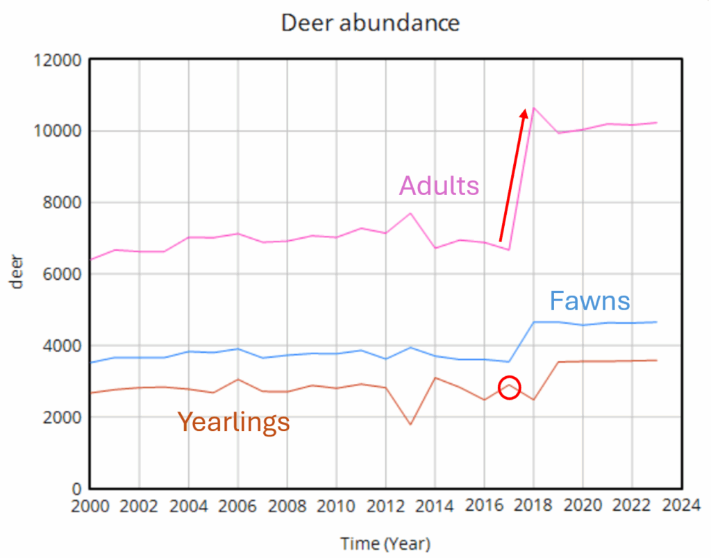
Deer populations have age structures. Fawns are born, in a year they mature into (surprise!) yearlings, and in another year they mature to adults. So this year’s yearlings are next year’s adults. But in the plot above, the increase in the adult data is about 4000 deer (red arrow), while the total yearling population aging into the adult category is about 3000. So the adult trajectory is simply impossible without negative mortality or an alien airdrop of 1000 extra deer into the county. Obviously this is an artifact of the methods change.
Once you’re aware of the age structure issue, other questionable features of the population data surface. For example, if you impose a one-year birth bonanza on a reduced form model, you see that births can’t produce a simple monotonic jump in population.
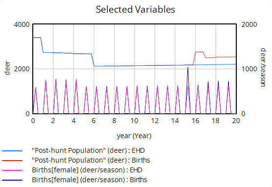
Instead, population spikes up, but falls back almost halfway to its initial level. This is because the spike of new fawns doesn’t immediately produce more births; fawns have a very low birth rate, so they have to mature through yearlings to adults before they make a substantial contribution to future population. Again if you look into the age structure, you can see these effects:

The bottom line is that abrupt increases in population are not very plausible – the dynamics just impose too many constraints.
In this modeling project, that means we’re in a bit of a pickle. Population dynamics have important interactions with CWD, but we don’t have reliable population measurements. The only option left to us is to do a lot of scenario analysis to try to capture the uncertain effects of various plausible trajectories.