The alien Hail Mary, and other climate policy plays

Cap & Trade is suspended in Europe and dead in the US, and the techno delusion may not be far behind. Some strange bedfellows have lined up behind the idea of R&D-driven climate policy. But now it appears that clean energy research is not a bipartisan no-brainer after all. Energy committee member Rand Paul’s bill would not only cut energy R&D funding by eliminating DOE altogether, it would cut our ability to even monitor the global environment by gutting NOAA and NASA. That only leaves one option:

13 In the otherwise dull year 2327, mankind successfully contacts aliens. Well, technically their answering machine, as the aliens themselves have gone to Alpha Centauri for the summer.

14 Desperate for help, humans leave increasingly stalker-y messages, turning off the aliens with how clingy our species is.

15 The aliens finally agree to equip Earth with a set of planet-saving carbon neutralizers, but work drags on as key parts must be ordered from a foreign supplier in the Small Magellanic Cloud.

16 The job comes in $3.7 quadrillion above estimate. Humanity thinks it is being taken advantage of but isn’t sure.

“20 things you didn’t know about the future,” in Discover

Seriously, where does that leave us? In terms of what we should do, I don’t think much has changed. As I wrote a while back, the climate policy table needs four legs:

  1. Prices
  2. Technology (the landscape of possibilities on which we make decisions)
  3. Institutional rules and procedures
  4. Preferences, operating within social networks

Preferences and technology are really the fundamentals among the four. Technology represents the set of options available to us for transforming energy and resources into life and play. Preferences guide how we choose among those options. Prices and rules are really just the information signals that allow us to coordinate those decisions.

However, neither preferences nor technology are as fundamental as they look. Models generally take preferences as a given, but in fact they’re endogenous. What we want on a day to day basis is far removed from our most existential needs. Instead, we construct preferences on the basis of technologies we know about, prices, rules, and the preferences and choices of others. That creates norms, fads, marketing, keep-up-with-the Joneses and other positive feedback mechanisms. Similarly, technology is more than discovery of principles and invention of devices. Those innovations don’t do anything until they’re woven into the fabric of society, guided by (you guessed it), prices, institutions, and preferences. That creates more positive feedbacks, like the chicken-egg problems of alternative fuel vehicle deployment.

If we could all get up in the morning and work out in our heads how to make Pareto-efficient decisions, we might not need prices and institutions, but we can’t, so we do. Prices matter because they’re a primary carrier of information through the economy. Not every decision is overtly economic, so we also have institutions, rules and routinized procedures to guide behavior. The key is that these signals should serve our values (the deeply held ones we’d articulate upon reflection, which might differ from the preferences revealed by transactions), not the other way around.

Preferences clearly can have a lot of direct leverage on behavior – if we all equated driving a big gas guzzler with breaking wind in a crowded elevator, we’d probably see different cars on the lot. However, most decisions are not so transparent. It’s already hard to choose “paper or plastic?” How about “desktop or server?” When you add multiple layers of supply chain and varied national origins to the picture, it becomes very hard to create a green information system paralleling the price system. It’s probably even harder to get individuals and firms to conform to such a system, when there are overwhelming evolutionary rewards to defection. Borrowing from Giraudoux, the secret to success is sustainability; once you can fake that you’ve got it made.

Similarly, the sheer complexity of society makes it hard to predict which technologies constitute a winning combination for creating low-carbon happiness. A technology-led strategy runs the risk of failing in the attempt to recreate a high-carbon lifestyle with low-carbon inputs.  I don’t think anyone has the foresight to select that portfolio. Even if we could do it, there’s no guarantee that, absent other signals, new technologies will be put to their intended uses, or that they will survive the “valley of death” between R&D and commercialization. It’s like airdropping a tyrannosaurus into an arctic ecosystem – sure, he’s got big teeth, but will he survive?

Complexity also militates against a rules-led approach. It’s simply too cumbersome to codify a rich set of tradeoffs in command-and-control regulations, which can become an impediment to innovation and are subject to regulatory capture. Also, systems like the CAFE standard create shadow prices of compliance, rather than explicit prices. This makes it hard to diagnose the effects of constraints and to coordinate them with other policies. There’s a niche for rules, but they shouldn’t be the big stick (on the other hand, eliminating the legacy of some past measures could be a win-win).

That’s why emissions pricing is really a keystone policy. Once you have prices aligned with the long term value of stable climate (and other resources), it’s easier to align the other legs of the table. Emissions prices create huge incentives for private R&D, leaving a smaller gap for government to fill – just the market failures in appropriation of benefits of technology. The points of pain where institutions are inadequate, or stand in the way of progress, will be more evident and easier to correct, and there will be less burden on policy making institutions, because they won’t have to coordinate many small programs to do the job of one big signal. Preferences will start evolving in a low-carbon direction, with rewards to those who (through luck or altruism) have already done so. Most importantly, emissions pricing gets some changes moving now, not after a decade or two of delay.

Concretely, I still think an upstream, revenue-neutral carbon tax is a practical implementation route. If there’s critical mass among trade partners, it could even evolve into a harmonized global system through the pressure of border carbon adjustments. The question is, how to get started?

Knowing Sooner

SEED magazine recently published an article on models for managing complex systems. In it, I talk about the C-ROADS experience. It nicely captures the punchline:

having the capacity to accurately predict the utility of proposed policy—whether it be domestic legislature or multilateral agreements—in real time while discussions are ongoing, opens the door for an entirely new way to enact policy.

I get too much credit for C-ROADS in the article; here are some of the people who really made it happen:

CI teamThe ClimateInteractive team: Travis Franck, Drew Jones, Stephanie McCauley, Phil Sawin, Beth Sawin, and Lori Siegel. Many other partners have also been instrumental, including John Sterman (MIT), Peter Senge (SOL), and really too many others to mention.

And so it begins…

A kerfuffle is brewing over Richard Tol’s FUND model (a recent  installment). I think this may be one of the first instances of something we’ll see a lot more of: public critique of integrated assessment models.

Integrated Assessment Models (IAMs) are a broad class of tools that combine the physics of natural systems (climate, pollutants, etc.) with the dynamics of socioeconomic systems. Most of the time, this means coupling an economic model (usually dynamic general equilibrium or an optimization approach; sometimes bottom-up technical or a hybrid of the two) with a simple to moderately complex model of climate. The IPCC process has used such models extensively to generate emissions and mitigation scenarios.

Interestingly, the IAMs have attracted relatively little attention; most of the debate about climate change is focused on the science. Yet, if you compare the big IAMs to the big climate models, I’d argue that the uncertainties in the IAMs are much bigger. The processes in climate models are basically physics and many are even be subject to experimental verification. We can measure quantities like temperature with considerable precision and spatial detail over long time horizons, for comparison with model output. Some of the economic equivalents, like real GDP, are much slipperier even in their definitions. We have poor data for many regions, and huge problems of “instrumental drift” from changing quality of goods and sectoral composition of activity, and many cultural factors are not even measured. Nearly all models represent human behavior – the ultimate wildcard – by assuming equilibrium, when in fact it’s not clear that equilibrium emerges faster than other dynamics change the landscape on which it arises. So, if climate skeptics get excited about the appropriate centering method for principal components analysis, they should be positively foaming at the mouth over the assumptions in IAMs, because there are far more of them, with far less direct empirical support.

Last summer at EMF Snowmass, I reflected on some of our learning from the C-ROADS experience (here’s my presentation). One of the key points, I think, is that there is a huge gulf between models and modelers, on the one hand, and the needs and understanding of decision makers and the general public on the other. If modelers don’t close that gap by deliberately translating their insights for lay audiences, focusing their tools on decision maker needs, and embracing a much higher level of transparency, someone else will do that translation for them. Most likely, that “someone else” will be much less informed, or have a bigger axe to grind, than the modelers would hope.

With respect to transparency, Tol’s FUND model is further along than many models: the code is available. So, informed tinkerers can peek under the hood if they wish. However, it comes with a warning:

It is the developer’s firm belief that most researchers should be locked away in an ivory tower. Models are often quite useless in unexperienced hands, and sometimes misleading. No one is smart enough to master in a short period what took someone else years to develop. Not-understood models are irrelevant, half-understood models treacherous, and mis-understood models dangerous.

Therefore, FUND does not have a pretty interface, and you will have to make to real effort to let it do something, let alone to let it do something new.

I understand the motivation for this warning. However, it leaves the modeler-consumer gulf gaping.The modelers have their insights into systems, the decision makers have their problems managing those systems, and ne’er the twain shall meet – there just aren’t enough modelers to go around. That leaves reports as the primary conduit of information from model to user, which is fine if your ivory tower is secure enough that you need not care whether your insights have any influence. It’s not even clear that reports are more likely to be understood than models: there have been a number of high-profile instances of ill-conceived institutional press releases and misinterpretation of conclusions and even raw data.

Also, there’s a hint of danger in the very idea of building dangerous models. Obviously all models, like analogies, are limited in their fidelity and generality. It’s important to understand those limitations, just as a pilot must understand the limitations of her instruments. However, if a model is a minefield for the uninitiated user, I have to question its utility. Robustness is an important aspect of model quality; a model given vaguely realistic inputs should yield realistic outputs most of the time, and a model given stupid inputs should generate realistic catastrophes. This is perhaps especially true for climate, where we are concerned about the tails of the distribution of possible outcomes. It’s hard to build a model that’s only robust to the kinds of experiments that one would like to perform, while ignoring other potential problems. To the extent that a model generates unrealistic outcomes, the causes should be traceable; if its not easy for the model user to see in side the black box, then I worry that the developer won’t have done enough inspection either. So, the discipline of building models for naive users imposes some useful quality incentives on the model developer.

IAM developers are busy adding spatial resolution, technical detail, and other useful features to models. There’s comparatively less work on consolidation of insights, with translation and construction of tools for wider consumption. That’s understandable, because there aren’t always strong rewards for doing so. However, I think modelers ignore this crucial task at their future peril.

What do SD bibliography entries say about the health of the field?

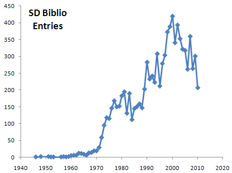
Here’s a time series of the number of entries in the system dynamics bibliography:

SD bibliography entries

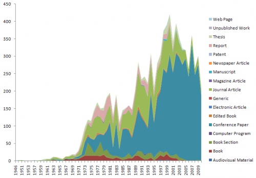
The peak was in 2000 with 420 entries. If you break out the types, it looks like the conference has saturated at about 250-300 papers, while journal, report and book publications have fallen off.

SD biblio detailI suspect that some of the decline is explained by a long reporting lag, and some is “defection” of SD work into journals that aren’t captured in the bibliography (probably a good thing). It would be interesting to see a corrected series, to see what it says about the health of the field. The ideal way to do the correction would be to build a simple dynamic model of actual and measured publication rates, estimating the parameters from data (student project, anyone?).

How Many Pairs of Rabbits Are Created by One Pair in One Year?

The Fibonacci numbers are often illustrated geometrically, with spirals or square tilings, but the nautilus is not their origin. I recently learned that the sequence was first reported as the solution to a dynamic modeling thought experiment, posed by Leonardo Pisano (Fibonacci) in his 1202 masterpiece, Liber Abaci.

How Many Pairs of Rabbits Are Created by One Pair in One Year?

A certain man had one pair of rabbits together in a certain enclosed place, and one wishes to know how many are created from the pair in one year when it is the nature of them in a single month to bear another pair, and in the second month those born to bear also. Because the abovewritten pair in the first month bore, you will double it; there will be two pairs in one month. One of these, namely the first, bears in the second month, and thus there are in the second month 3 pairs; of these in one month two are pregnant, and in the third month 2 pairs of rabbits are born, and thus there are 5 pairs in the month; in this month 3 pairs are pregnant, and in the fourth month there are 8 pairs, of which 5 pairs bear another 5 pairs; these are added to the 8 pairs making 13 pairs in the fifth month; these 5 pairs that are born in this month do not mate in this month, but another 8 pairs are pregnant, and thus there are in the sixth month 21 pairs; [p284] to these are added the 13 pairs that are born in the seventh month; there will be 34 pairs in this month; to this are added the 21 pairs that are born in the eighth month; there will be 55 pairs in this month; to these are added the 34 pairs that are born in the ninth month; there will be 89 pairs in this month; to these are added again the 55 pairs that are born in the tenth month; there will be 144 pairs in this month; to these are added again the 89 pairs that are born in the eleventh month; there will be 233 pairs in this month.

Source: http://www.math.utah.edu/~beebe/software/java/fibonacci/liber-abaci.html

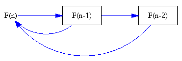
The solution is the famous Fibonacci sequence, which can be written as a recurrent series,

F(n) = F(n-1)+F(n-2), F(0)=F(1)=1

This can be directly implemented as a discrete time Vensim model:

Fibonacci SeriesHowever, that representation is a little too abstract to immediately reveal the connection to rabbits. Instead, I prefer to revert to Fibonacci’s problem description to construct an operational representation:
Fibonacci Rabbits

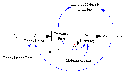
Mature rabbit pairs are held in a stock (Fibonacci’s “certain enclosed space”), and they breed a new pair each month (i.e. the Reproduction Rate = 1/month). Modeling male-female pairs rather than individual rabbits neatly sidesteps concern over the gender mix. Importantly, there’s a one-month delay between birth and breeding (“in the second month those born to bear also”). That delay is captured by the Immature Pairs stock. Rabbits live forever in this thought experiment, so there’s no outflow from mature pairs.

You can see the relationship between the series and the stock-flow structure if you write down the discrete time representation of the model, ignoring units and assuming that the TIME STEP = Reproduction Rate = Maturation Time = 1:

Mature Pairs(t) = Mature Pairs(t-1) + Maturing
Immature Pairs(t) = Immature Pairs(t-1) + Reproducing - Maturing

Substituting Maturing = Immature Pairs and Reproducing = Mature Pairs,

Mature Pairs(t) = Mature Pairs(t-1) + Immature Pairs(t-1)
Immature Pairs(t) = Immature Pairs(t-1) + Mature Pairs(t-1) - Immature Pairs(t-1) = Mature Pairs(t-1)

So:

Mature Pairs(t) = Mature Pairs(t-1) + Mature Pairs(t-2)

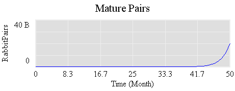
The resulting model has two feedback loops: a minor negative loop governing the Maturing of Immature Pairs, and a positive loop of rabbits Reproducing. The rabbit population tends to explode, due to the positive loop:

Fibonacci Growth

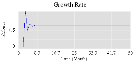
In four years, there are about as many rabbits as there are humans on earth, so that “certain enclosed space” better be big. After an initial transient, the growth rate quickly settles down:

Fibonacci Growth RateIts steady-state value is .61803… (61.8%/month), which is the Golden Ratio conjugate. If you change the variable names, you can see the relationship to the tiling interpretation and the Golden Ratio:
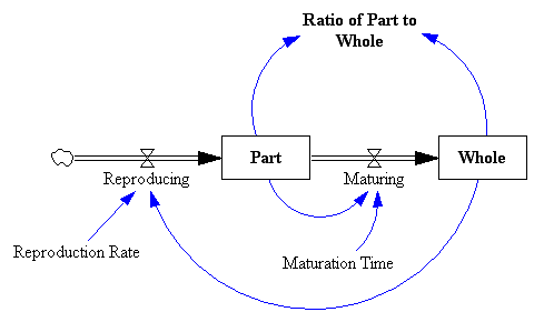
Fibonacci Part Whole

Like anything that grows exponentially, the Fibonacci numbers get big fast. The hundredth is  354,224,848,179,261,915,075.

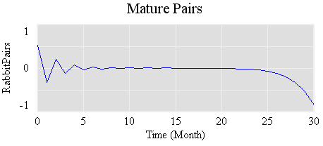
As before, we can play the eigenvector trick to suppress the growth mode. The system is described by the matrix:

-1 1
 1 0

which has eigenvalues {-1.618033988749895, 0.6180339887498949} – notice the appearance of the Golden Ratio. If we initialize the model with the eigenvector of the negative eigenvalue, {-0.8506508083520399, 0.5257311121191336}, we can get the bunny population under control, at least until numerical noise excites the growth mode, near time 25:

Fibonacci Stable

The problem is that we need negarabbits to do it, -.850653 immature rabbits initially, so this is not a physically realizable solution (which probably guarantees that it will soon be introduced in legislation).

I brought this up with my kids, and they immediately went to the physics of the problem: “Rabbits don’t live forever. How big is your cage? Do you have rabbit food? TONS of rabbit food? What if you have all males, or varying mixtures of males and females?”

It’s easy to generalize the structure to generate other sequences. For example, assuming that mature rabbits live for only two months yields the Padovan sequence. Its equivalent of the Golden Ratio is 1.3247…, i.e. the rabbit population grows more slowly at ~32%/month, as you’d expect since rabbit lives are shorter.

The model’s in my library.

Fibonacci Rabbits

This is a small, discrete time model that explores the physical interpretation of the Fibonacci sequence. See my blog post about this model for details.

Fibonacci2.vpm This runs with Vensim PLE, but users might want to use the Model Reader in order to load the included .cin file with non-growing eigenvector settings.

The simple dynamics of violence

There’s simple, as in Occam’s Razor, and there’s simple, as in village idiot.

There’s a noble tradition in economics of using simple thought experiments to illuminate important dynamics. Sometimes things go wrong, though, like this (from a blog I usually like):

… suppose that you have the choice of providing gruesome rhetoric that will increase the probability of a killing spree but will also increase the probability of the passage of Universal Health Insurance. Suppose using the Arizona case as a baseline we say that the average killing spree causes the death of 6 people. Then if your rhetoric is at least 6/22,000 = 1/3667 times as likely to produce a the passage of universal health insurance as it is to induce a killing spree then you saved lives by engaging in fiery rhetoric.

http://modeledbehavior.com/2011/01/11/the-optimal-quantity-of-violent-rhetoric/

Here’s the apparent mental model behind this reasoning:

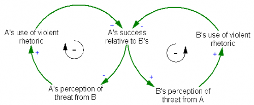
Linear ViolenceIt’s linear: use violent rhetoric, get the job done. There are two problems with this simple model. First, the sign of the relationships is ambiguous. I tend to suspect that anyone who needs to use violent rhetoric is probably a fanatic, who shouldn’t be making policy in the first place. Setting that aside, the bigger problem is that violence isn’t linear. Like potato chips, you can never have just one excessive outburst. Violent rhetoric escalates, and sometimes crosses into real violence. This is the classic escalation archetype:

Violence EscalationIn the escalation archetype, two sides struggle to maintain an advantage over each other. This creates two inner negative feedback loops, which together create a positive feedback loop (a figure-8 around the two negative loops). It’s interesting to note that, so far, the use of violent rhetoric is fairly one-sided – the escalation is happening within the political right (candidates vying for attention?) more than between left and right.
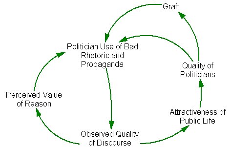
There are many other positive feedbacks involved in the process, which exacerbate the direct escalation of language. Here are some speculative examples:

Violence Other LoopsThe positive feedbacks around violent rhetoric create a societal trap, from which it may be difficult to extricate ourselves. If there’s a general systems insight about vicious cycles, it’s that the best policy is prevention – just don’t start down that road (if you doubt this, play the dollar auction or smoke some crack). Politicians who engage in violent rhetoric, or other races to the bottom of the intellectual barrel, risk starting a very destructive spiral:
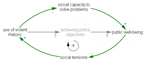
violence Social

The bad news is that there’s no easy remedy for this behavior. Purveyors of violent rhetoric and their supporters need to self-reflect on the harm they do to society. The good news is that if public support for violent words and images reverses, the positive loops will help to repair the damage, and take us closer to a model of rational discourse for problem solving.

About that, there is at least a bit of wisdom in the article:

… if you genuinely care about the shooting death of six people then you ought to really, really care about endorsing wrong public policies which will result in the premature death of vastly more people. Hence you should devote yourself to actually discovering the right answers to these questions, rather than than coming up with ad hoc rhetoric – violent or polite – in support of the policy you happend to have been attracted to first.

Optimizing Vensim models

Danger – another technical post, mainly relevant to users of advanced Vensim versions.

The title has a double meaning: I’m talking about optimizing the speed of a model, which is most often needed for optimization problems.

Here’s the challenge: you have a model, and you think you understand it. You’d like to calibrate it to data, do some policy optimization to identify good decision rules, and do some Monte Carlo simulation to identify sensitive parameters and robust policies. All of those things take thousands or even millions of model runs. Or, maybe you’d just like to make a slightly sluggish model fast enough to run interactively with Synthesim.

Here’s what you can do:

  • Run compiled. Probably your best bet is to use MS Visual c++ 2010 Express, which is free, or an old copy of MSVC 6. Some of the versions in between apparently have problems. You may need to change Vensim’s mdl.bat file to match the specific paths of your software. You might succeed with free tools, like gcc+, but I haven’t tried – I’d be interested to hear of such adventures. Update: You now want Visual Studio with the C/C++ workload. For recent versions of Vensim, it’s actually mdldp64.bat that contains the active compile script. It usually works right out of the box.
  • Use the INITIAL() statement as much as you can. In particular, be sure that any data-retrieval functions like GET DATA AT TIME are wrapped in an initial if possible (they’re comparatively slow).
  • Consider using data equations for input calculations that are not part of the feedback structure of the model. Data equations get executed once, at the start of a group of optimization/sensitivity/Synthesim simulations, rather than with each iteration. However, don’t use data equations where parameters you plan to change are involved, because then your changes won’t propagate through the results. If you want to save startup time too, move complex data calculations into an offline data model.
  • Switch any sparse array summary calculations from SUM, VMIN, VMAX, and PROD functions to VECTOR SELECT or VECTOR ELM MAP. Update: I’m no longer sure this is worth the trouble.
  • Update: Calculate vector sums only once. For example, instead of writing share[k] = quantity[k]/SUM(quantity[k!]), calculate the sum separately, so that share[k] = quantity[k]/total quantity and  total quantity = SUM(quantity[k!]).
  • Get rid of any extraneous structure that’s not related to your payoff or other variables of interest. If you still want the information, move it to a separate model that reads the main model’s .vdf for postprocessing. Update: you can put it in a submodel and load it, or not, as needed.
  • Consider whether your payoff is separable. In other words, if your model boils down to payoff = part1(parameter1) + part2(parameter2), you can optimize sequentially for parameter1 and parameter2, since they don’t interact. Vensim’s algorithm is designed for the worst case – parameters that interact, multiple optima, discontinuities, etc. You can automate a sequential set of optimizations with a command script.
  • Consider transforming some of your optimization parameters. For example, if you are fitting to data for a stock with a first order outflow, that outflow can be written as stock/tau or stock*delta, where tau and delta are the lifetime and fractional loss rate, respectively. Mathematically, it makes no difference whether you use the tau or delta approach, but in some practical cases it might. For example, if you think delta might be near zero (a long lifetime), you might do better to optimize over delta = [0,1] than tau = [1,1e9].
  • If you’re looking for hardware improvements, clock speed matters more than multicores and cache. Update: for optimization, MCMC and sensitivity runs, multiple cores help a lot in v10+.

These options are in the order that I thought of them, which means that they’re very roughly in order of likely improvement per unit effort.

Unfortunately, it’s often the case that all of this will get you a 10x improvement, and you need 1000x. Unless you have a supercomputer or massive parallel grid at your disposal, the only real remedy is to simplify your model. Fortunately, that’s not necessarily a bad thing.

Update: One more thing to try: if you’re doing single simulations with a large model, the bottleneck may be the long disk write of the output .vdf file. In that case, you can use a savelist (.lst) to restrict the number of variables stored to just the output you’re interested in. However, you should occasionally do a run without a savelist, and browse through the model results to be sure that things are OK. Consider writing some Reality Checks to enforce quality control on things you won’t be looking at.

Update 2: Another suggestion, via Hazhir Rahmandad: when using the ALLOC functions (DEMAND AT PRICE, etc.), choose simple demand/supply function shapes, like triangular, rather than complex shapes like exponential. The allocation functions iterate to equilibrium internally, and this can be time consuming. Avoiding the use of FIND ZERO and SIMULTANEOUS where possible is also helpful – often a lookup or polynomial approximation to the solution of simultaneous equations will suffice.

The rebound delusion

Lately it’s become fashionable to claim that energy efficiency is useless, because the rebound effect will always eat it up. This is actually hogwash, especially in the short term. James Barrett has a nice critique of the super-rebound position at RCE. Some excerpts:

To be clear, the rebound effect is real. The theory behind it is sound: Lower the cost of anything and people will use more of it, including the cost of running energy consuming equipment. But as with many economic ideas that are sound theory (like the idea that you can raise government revenues by cutting tax rates), the trick is in knowing how far to take them in reality. (Cutting tax rates from 100% to 50% would certainly raise revenues. Cutting them from 50% to 0% would just as surely lower them.)

The problem with knowing how far to take things like this is that unlike real scientists who can run experiments in a controlled laboratory environment, economists usually have to rely on what we can observe in the real world. Unfortunately, the real world is complicated and trying to disentangle everything that’s going on is very difficult.

Owen cleverly avoids this problem by not trying to disentangle anything.

One supposed example of the Jevons paradox that he points to in the article is air conditioning. Citing a conversation with Stan Cox, author of Losing Our Cool, Owen notes that between 1993 and 2005, air conditioners in the U.S. increased in efficiency by 28%, but by 2005, homes with air conditioning increased their consumption of energy for their air conditioners by 37%.

Accounting only for the increased income over the timeframe and fixing Owen’s mistake of assuming that every air conditioner in service is new, a few rough calculations point to an increase in energy use for air conditioning of about 30% from 1993 to 2005, despite the gains in efficiency. Taking into account the larger size of new homes and the shift from room to central air units could easily account for the rest.

All of the increase in energy consumption for air conditioning is easily explained by factors completely unrelated to increases in energy efficiency. All of these things would have happened anyway. Without the increases in efficiency, energy consumption would have been much higher.

It’s easy to be sucked in by stories like the ones Owen tells. The rebound effect is real and it makes sense. Owen’s anecdotes reinforce that common sense. But it’s not enough to observe that energy use has gone up despite efficiency gains and conclude that the rebound effect makes efficiency efforts a waste of time, as Owen implies. As our per capita income increases, we’ll end up buying more of lots of things, maybe even energy. The question is how much higher would it have been otherwise.

Why is the rebound effect suddenly popular? Because an overwhelming rebound effect is needed to make sense of proposals to give up on near-term emissions prices and invest in technology, praying for a clean-energy-supply miracle in a few decades.

As Barrett points out, the notion that energy efficiency increases energy use is an exaggeration of the rebound effect. For efficiency to increase use, energy consumption has to be elastic (e<-1). I don’t remember ever seeing an economic study that came to that conclusion. In a production function, such values aren’t physically plausible, because they imply zero energy consumption at a finite energy price.

Therefore, the notion that pursuing energy efficiency makes the climate situation worse is a fabrication. Doubly so, because of an accounting sleight-of-hand. Consider two extremes:

  1. no rebound effects (elasticity ~ 0): efficiency policies work, because they reduce energy use and its associated negative social externalities.
  2. big rebound effects (elasticity < -1): efficiency policies increase energy use, but they do so because there’s a huge private benefit from the increase in mobility or illumination or whatever private purpose the energy is put to.

The super-rebound crowd pooh-poohs #1 and conveniently ignores the welfare outcome of #2, accounting only for the negative side effects.

If rebound effects are modest, as they surely are, it makes much more sense to guide R&D and deployment for both energy supply and demand with a current price signal on emissions. That way, firms make distributed decisions about where to invest, rather than the government picking winners, and appropriate tradeoffs between conservation and clean supply are possible. The price signal can be adapted to meet environmental constraints in the face of rising income. Progress starts now, rather than after decades of waiting for the discover->apply->deploy->embody pipeline.

If the public isn’t ready for it, that doesn’t mean analysts should bargain against their own good sense by recommending things that might be popular, but are unlikely to work. That’s like a doctor advising a smoker to give to cancer research, without mentioning that he really ought to quit.

Update: there’s an excellent followup at RCE.