This started out as a techy post about infection models for SD practitioners interested in epidemiology. However, it has turned into something more important for coronavirus policy.
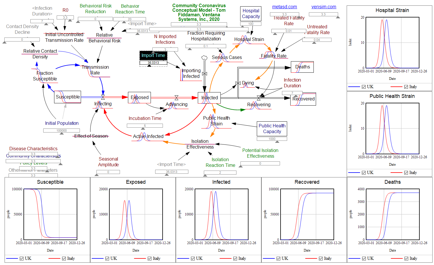
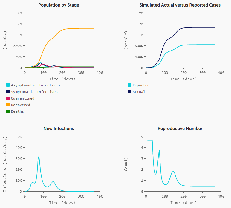
It began with a puzzle: I re-implemented my conceptual coronavirus model for multiple regions, tuning it for Italy and Switzerland. The goal was to use it to explore border closure policies. But calibration revealed a problem: using mainstream parameters for the incubation time, recovery time, and R0 yielded lukewarm growth in infections. Retuning to fit the data yields R0=5, which is outside the range of most estimates. It also makes control extremely difficult, because you have to reduce transmission by 1-1/R0 = 80% to stop the spread.
To understand why, I decided to solve the model analytically for the steady-state growth rate in the early infection period, when there are plenty of susceptible people, so the infection rate is unconstrained by availability of victims. That analysis is reproduced in the subsequent sections. It’s of general interest as a way of thinking about growth in SD models, not only for epidemics, but also in marketing (the Bass Diffusion model is essentially an epidemic model) and in growing economies and supply chains.
First, though, I’ll skip to the punch line.
The puzzle exists because R0 is not a complete description of the structure of an epidemic. It tells you some important things about how it will unfold, like how much you have to reduce transmission to stop it, but critically, not how fast it will go. That’s because the growth rate is entangled with the incubation and recovery times, or more generally the distribution of the generation time (the time between primary and secondary infections).
This means that an R0 value estimated with one set of assumptions about generation times (e.g., using the R package R0) can’t be plugged into an SEIR model with different delay structure assumptions, without changing the trajectory of the epidemic. Specifically, the growth rate is likely to be different. The growth rate is, unfortunately, pretty important, because it influences the time at which critical thresholds like ventilator capacity will be breached.
The mathematics of this are laid out clearly by Wallinga & Lipsitch. They approach the problem from generating functions, which give up simple closed-form solutions a little more readily than my steady-state growth calculations below. For example, for the SEIR model,
R0 = (1 + r/b1)(1 + r/b2) (Eqn. 3.2)
Where r is the growth rate, b1 is the inverse of the incubation time, and b2 is the inverse of the recovery time. If you plug in r = 0.3/day, b1 = 1/(5 days), b2 = 1/(10 days), R0 = 10, which is not plausible for COVID-19. Similarly, if you plug in the frequently-seen R0=2.4 with the time constants above, you get growth at 8%/day, not the observed 30%/day.
There are actually more ways to get into trouble by using R0 as a shorthand for rich assumptions in models. Stochastic dynamics and network topology matter, for example. In The Failure of R0, Li Blakely & Smith write,
However, in almost every aspect that matters, R 0 is flawed. Diseases can persist with R 0 < 1, while diseases with R 0 > 1 can die out. We show that the same model of malaria gives many different values of R 0, depending on the method used, with the sole common property that they have a threshold at 1. We also survey estimated values of R 0 for a variety of diseases, and examine some of the alternatives that have been proposed. If R 0 is to be used, it must be accompanied by caveats about the method of calculation, underlying model assumptions and evidence that it is actually a threshold. Otherwise, the concept is meaningless.
Is this merely a theoretical problem? I don’t think so. Here’s how things stand in some online SEIR-type simulators:
| Model | R0 (dmnl) | Incubation (days) | Infectious (days) | Growth Rate (%/day) |
| My original | 3.3 | 5 | 7 | 17 |
| Homer US | 3.5 | 5.4 | 11 | 18 |
| covidsim.eu | 4 | 4 & 1 | 10 | 17 |
| Epidemic Calculator | 2.2 | 5.2 | 2.9 | 30* |
| Imperial College | 2.4 | 5.1 | ~3** | 20*** |
*Observed in simulator; doesn’t match steady state calculation, so some feature is unknown.
**Est. from 6.5 day mean generation time, distributed around incubation time.
***Not reported; doubling time appears to be about 6 days.
I think this is certainly a Tower of Babel situation. It seems likely that the low-order age structure in the SEIR model is problematic for accurate representation of the dynamics. But it also seems like piecemeal parameter selection understates the true uncertainty in these values. We need to know the joint distribution of R0 and the generation time distribution in order to properly represent what is going on.