The Mysterious TREND Function

This post is literally trending.

Most System Dynamics software includes a pair of TREND and FORECAST functions. For historic reasons, these are typically the simplest possible first-order structure, which is fine for continuous, deterministic models, but not the best for applications with noise or real data. The waters are further muddied by the fact that Excel has a TREND function that’s really FORECASTing, plus newer FORECAST functions with methods that may differ from typical SD practice. Business Dynamics describes a third-order TREND function that’s considerably better for real-world applications.

As a result of all this variety, I think trend measurement and forecasting remain unnecessarily mysterious, so I built the model below to compare several approaches.

Goal

The point of TREND and FORECAST functions is to model the formation of expectations in a way that closely matches what people in the model are really doing.

This could mean a wide variety of things. In many cases, people aren’t devoting formal thought to observing and predicting the phenomenon of interest. In that case, adaptive expectations may be a good model. The implementation in SD is the SMOOTH function. Using a SMOOTH to set expectations says that people expect the future to be like the past, and they perceive changes in conditions only gradually. This is great if the forecasted variable is in fact stationary, or at least if changes are slow compared to the perception time. On the other hand, for a fast-evolving situation like COVID19, delay can be fatal – literally.

For anything that is in fact changing (or that people perceive to be changing), it makes sense to project changes into the future with some kind of model. For a tiny fraction of reality, that might mean a sophisticated model: multiple regression, machine learning, or some kind of calibrated causal model, for example. However, most things are not subject to that kind of sophisticated scrutiny. Instead, expectations are likely to be formed by some kind of simple extrapolation of past trends into the future.

In some cases, things that are seemingly modeled in a sophisticated way may wind up looking a lot like extrapolation, due to human nature. The forecasters form a priori expectations of what “good” model projections look like, based on fairly naive adaptive-extrapolative expectations and social processes, and use those expectations to filter the results that are deemed acceptable. This makes the sophisticated results look a lot like extrapolation. However, the better the model, the harder it is for this to happen.

More Oil Price Forecasts

The goal, by the way, is generally not to use trend-like functions to make a forecast. Extrapolation may be perfectly reasonable in some cases, particularly where you don’t care too much about the outcome. But generally, you’re better off with a more sophisticated model – the whole point of SD and other methods is to address the feedback and nonlinearities that make extrapolation and other simpleminded methods go wrong. On the other hand, simple extrapolation may be great for creating a naive or null forecast to use as a benchmark for comparison with better approaches.

Basics

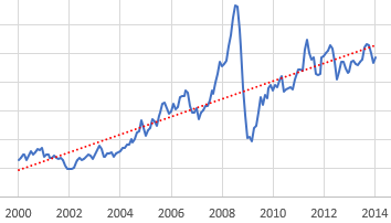
So, let’s suppose you want to model the expectations for something that people perceive to be (potentially) steadily increasing or decreasing. You can visit St. Louis FRED and find lots of economic series like this – GDP, prices, etc. Here’s the spot price of West Texas Intermediate crude oil:

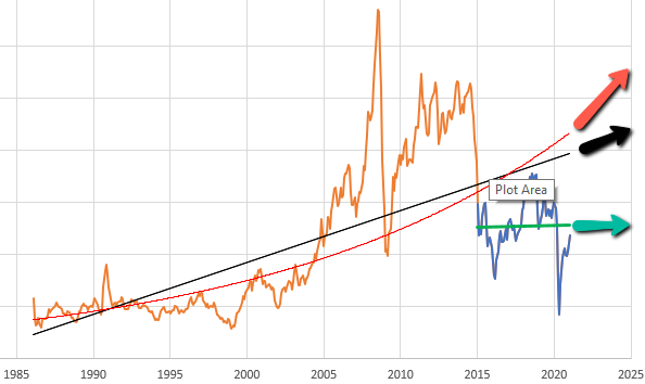
Given this data, there are immediately lots of choices. Thinking about someone today making an investment conditional on future oil prices, should they extrapolate linearly (black and green lines) or exponentially (red line)? Should they use the whole series (black and red) or just the last few years (green)? Each of these implies a different forecast for the future.

Suppose we have some ideas about the forecast horizon, desired sensitivity to noise, etc. How do we actually establish a trend? One option is linear regression, which is just a formal way of eyeballing a straight line that fits some data. It works well, but has some drawbacks. First, it assigns equal weight to all the data throughout the interval, and zero weight to anything outside the interval. That may be a poor model for perceptual processes, where the most recent data has the greatest salience to the decision maker. Second, it’s computation- and storage-intensive: you have to do a lot of math, and keep track of every data point within the window of interest. That’s fine if it resides in a spreadsheet, but not if it resides in someone’s head.

Linear fit to a subset of the WTI spot price data.

The trend-like functions make an elegant simplification that addresses the drawbacks of regression. It’s based on the following observation:*

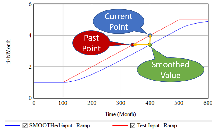
If, as above, you take a growing input (red line) and smooth it exponentially (using the SMOOTH function, or an equivalent first order goal-gap structure), you get the blue line: another ramp, that lags the input with a delay equal to the smoothing time. This means that, at month 400, we know two points: the current value of the input, and the current value of the smoothed input. But the smoothed value represents the past value of the input, in this case 60 months previous. So, we can use these two points to determine the slope of the red line:

(1) slope = (current - smoothed) / smoothing time

This is the slope in terms of input units per time. It’s often convenient to compute the fractional slope instead, expressing the growth as a fractional increase in the input per unit time:

(2) fractional slope = (current - smoothed) / smoothed / smoothing time

This is what the simple TREND functions in SD software typically report. Note that it blows up if the smoothed quantity reaches 0, while the linear method (1) does not.

If we think the growth is exponential, rather than a linear ramp, we can compute the growth rate in continuous time:

(3) fractional growth rate = LN( current / smoothed ) / smoothing time

This has pros and cons. Obviously, if a quantity is really growing exponentially, it should be measured that way. But if we’re modeling how people actually think, they may extrapolate linearly when the underlying behavior is exponential, thereby greatly underestimating future growth. Note that the very idea of forecasting exponentially assumes that the values involved are positive.

Once you know the slope of the (estimated) line, you can extrapolate it into the future via a method that corresponds with the measurement:

(1b) future value = current + slope * forecast horizon
(2b) future value = current * (1 + fractional slope * forecast horizon)
(3b) future value = current * EXP( fractional growth rate * forecast horizon )

Typical FORECAST functions use (2b).

*There’s a nice discussion of this in Appendix L of Industrial Dynamics, around figure L-3.

Refinements

The strategy above has the virtue of great simplicity: you only need to keep track of one extra stock, and the computation needed to extrapolate is minimal. It works great for continuous models. Unfortunately, it’s not very resistant to noise and discontinuities. Consider what happens if the input is not a smooth line, but a set of noisy points scattered around the line:

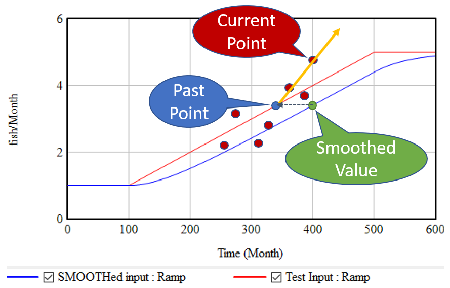
The SMOOTH function filters the data, so the past point (blue) may still be pretty close to the underlying input trend (red line). However, the extrapolation (orange line) relies only on the past point and the single current point. Any noise or discontinuity in the current point therefore can dramatically influence the slope estimate and future projections. This is not good.

Similar perverse behaviors happen if the input is a pulse or step function. For example:

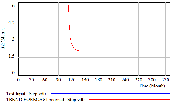
Fortunately, simple functions can be saved. In Expectation Formation in Behavioral Simulation Models, John Sterman describes an alternative third-order TREND function that improves robustness and realism. The same structure can be found in the excellent discussion of expectations in Business Dynamics, Chapter 16.

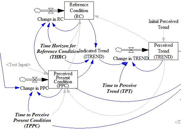
I’ll leave the details to the article, but the basic procedure is:

  • Recognize that the input is not perceived instantaneously, but only after some delay (represented by smoothing). This might capture the fact that formal accounting procedures only report results with a lag, or that you only see the price of cheese at the supermarket intermittently.
  • Track a historic point (the Reference Condition), by smoothing, as in the simpler methods.
  • Measure the Indicated Trend as the fractional slope between the Perceived Present Condition and the Reference Condition.
  • Smooth the Indicated Trend again to form the final Perceived Trend. The smoothing prevents abrupt changes in the indicated trend from causing dramatic overshoots or undershoots in the trend estimate and extrapolations that use it.

There’s an intermediate case that’s actually what I’m most likely to reach for when I need something like this: second-order smoothing. There are actually several very similar approaches (see double exponential smoothing for example) in the statistical literature. You have to be a little cautious, because these are often expressed in discrete time and therefore require a little thought to adapt to continuous time and/or unequal data intervals.

The version I use does the following:

(4) smoothed input = SMOOTH( input, smoothing time )

(5) linear trend = (input-smoothed input) / smoothing time
(6) smoothed trend = SMOOTH( linear trend, trend smoothing time )
(7) forecast = smoothed input + smoothed trend*(smoothing time + forecast horizon)

This provides most of what you want in a simple extrapolation method. It largely ignores a PULSE disturbance. Overshoot is mild when presented with a STEP input (as long as the smoothing times are long enough). It largely rejects noise, but still tracks a real RAMP accurately.

Back to regression

SD models typically avoid linear regression, for a reasons that are partly legitimate (as mentioned above). But it’s also partly cultural, as a reaction to incredibly stupid regressions that passed for models in other fields around the time of SD’s inception. We shouldn’t throw the baby out with that bathwater.

Fortunately, while most software doesn’t make linear regression particularly accessible, it turns out to be easy to implement an online regression algorithm with stocks and flows with no storage of data vectors required. The basic insight is that the regression slope (typically denoted beta) is given by:

(8) slope = covar(x,y) / var(x)

where x is time and y is the input to be forecasted. But var() and covar() are just sums of squares and cross products. If we’re OK with having exponential weighting of the regression, favoring more recent data, we can track these as moving sums (analogous to SMOOTHs). As a further simplification, as long as the smoothing window is not changing, we can compute var(x) directly from the smoothing window, so we only need to track the mean and covariance, yielding another second-order smoothing approach.

If the real decision makers inspiring your model are actually using linear regression, this may be a useful way to implement it. The implementation can be extended to equal weighting over a finite interval if needed. I find the second-order smoothing approach more intuitive, and it performs just as well, so I tend to prefer that in most cases.

Extensions

Most of what I’ve described above is linear, i.e. it assumes linear growth or decline of the quantity of interest. For a lot of things, exponential growth will be a better representation. Equations (3) and (3b) assume that, but any of the other methods can be adapted to assume exponential behavior by operating on the logarithm of the input, and then inverting that with exp(…) to form the final output.

All the models described here share one weakness: cyclical inputs.

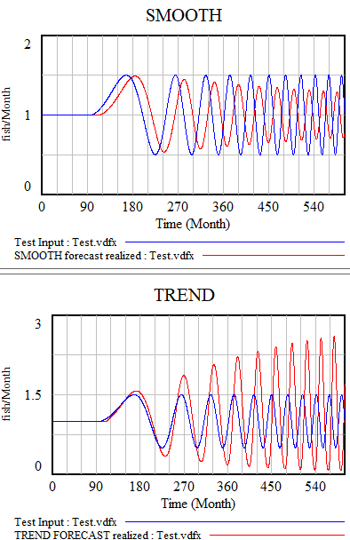
When presented with a sin wave, the simplest approach – smoothing – just bulldozes through. The higher the frequency, the less of the signal passes into the forecast. The TREND function can follow a wave if the period is longer than the smoothing time. If the dynamics are faster, it starts to miss the turning points and overshoot dramatically. The higher-order methods are better, but still not really satisfactory. The bottom line is that your projection method must use a model capable of representing the signal, and none of the methods above embodies anything about cyclical behavior.

There are lots of statistical approaches to detection of seasonality, which you can google. Many involve binning techniques, similar to those described in Appendix N of Industrial Dynamics, Self Generated Seasonal Cycles.

The model

The Vensim model, with changes (.cin) files implementing some different experiments:

trendy 4b.zip

I developed this in DSS and forgot to test PLE before uploading. If you have issues, please comment and I’ll adapt it to work.

A Ventity version is on the way.

Misadventures with Little’s Law

I’ve been working on a vehicle fleet model, re-implementing a spreadsheet in Ventity, using dynamic cohorts.

The vehicle lifetime in the spreadsheet is 11 years, and it’s discrete. This means that every vehicle retires precisely 11 years after it’s put into service. This raised a red flag for me, because it represents a rather short vehicle lifetime. I know from work in other jurisdictions that the average life of a vehicle is more like 16-18 years typically (and getting longer as quality improves).

So, where does the 11 year figure come from? We’re not sure. Other published data for the region indicates an average vehicle age of 8.5 years, so it’s not that. A Ventana colleague pointed out that it might be a steady-state estimate from combining vehicle fleet data with new vehicle sales data:


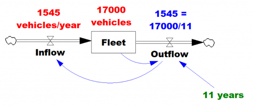
Given the data (red), assume that the vehicle stock is in equilibrium (inflow=outflow). Then it follows from
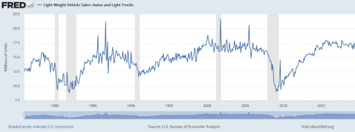
 Little’s Law that the average lifetime of vehicles must be 11 years. Little’s Law works regardless of the delay distribution, i.e. regardless of the delay order, but if you were formulating the fleet as a first-order system, that’s precisely how you’d write the outflow equation: outflow = fleet/lifetime, with lifetime=11 years.

… the long-term average number L of customers in a stationary system is equal to the long-term average effective arrival rate λ multiplied by the average time W that a customer spends in the system. – Wikipedia

However, there’s a danger here. The system might not be in equilibrium. Then both the assumption of inflow=0utflow and the stationarity required in Little’s Law. Vehicle sales are, unfortunately, rather volatile, particularly around events like the 2008 recession:

It’s tempting to use the average age of vehicles as another data point, but that turns out to be a bad idea. The average age of vehicles is sensitive to both variations in the inflow and the assumed distribution of the discard process. The following Ventity model illustrates this problem, using some of the same machinery as last week’s Erlang model.

As before, there’s a population of entities (agents). Each has a cascade of N internal states, represented by a stock counter, and an age that increases continuously. An entity deletes itself when it’s too old, or its state count is too high.

For accounting purposes, when an entity “dies” it records the event by incrementing counter stocks in the Model entity:

In this way, we can keep track of how old the average entity was at the time it deleted itself. This should be the average residence time in Little’s Law. We can also track the average age of existing entities, to see whether it’s the same.

First, consider a very simple, very nonstationary special case, in which there’s no flow of entity turnover. There’s only an initial population of entities of age 0, who gradually leave the system. Here are three variants of that experiment:

Set Model.Delay tau = 50 and Model.Flow Start Time = 1000 to replicate this experiment.

The blue line is the stochastic population analog of the classic first-order delay. The probability of a given entity departing is constant over time, as for radioactive decay. Therefore we get exponential decay, with count = N0*exp(-time/Delay tau). The red line is the third-order equivalent, yielding an Erlang 3 distribution. The green line is the pipeline delay equivalent, in which all entities self-delete at a specified age, rather than with a random distribution. Therefore the population steps from 1000 to 0 at time 50.

The two lower panels compare the average age of surviving entities (middle) to the average age at which entities self-delete (bottom). At bottom, you can see that all variants eventually converge to (roughly) the expected 50-year entity lifespan. However, each trajectory initially indicates a shorter lifespan. This is due to a form of censoring bias – at a given point in time, the longest-lived entities have not yet been observed.

The middle panel indicates how average age can mislead. In this case, age=time for all entities, and therefore the average age increases linearly, even though the expected residence time is constant.

At the opposite extreme, here’s an experiment with a constant flow of new agents, so that the system is in equilibrium after a few time constants:

Set Model.Delay tau = 20 and Model.Flow Start Time = 0 to replicate this experiment.

After the initial transient has died out (by time 20 to 60), all 3 residence times (age at deletion) converge to the expected value of 20. But notice the ages. They converge, too, but the value is dependent on the distribution. For the 1st-order system (blue), the average age does equal the average residence time of 20 years. But the pipeline system (green) has an average age that’s half that, at 10 years. This makes sense, if you think about an equilibrium population composed of a uniform mix of ages between 0 and 20 years. The 3rd-order system is in between.

This uncertain relationship between age and residence time means that we can’t use the average age of the vehicle fleet to determine the rate of vehicle turnover. That’s too bad, because age is the one statistic that’s easy to compute from a database of vehicle registrations. To know more, we have to start making inferences about the inflows and outflows – but that’s tricky if data coverage varies with time. Unfortunately, this is a number that we care about, because the residence time of vehicles in the system is an important driver of future penetration of low-carbon technologies.

The model: AgentAge2.zip

The Delay Sandbox can be used to explore similar phenomena in a continuous, aggregate, deterministic setting.

Aging Chains and the Erlang Distribution

My Delay Sandbox model illustrates the correspondence between Nth-order delays and the Erlang distribution (among other things).

Delay Sandbox

This model provides some similar insights – this time in Ventity. It’s a hybrid of classic continuous SD and agent equivalents.

First, the Erlang3 entitytype compares the classic 3rd-order aging chain’s behavior to analytical equivalents, as in the Delay Sandbox. The analytic values are computed in a set of Ventity’s new macros:

Notice that the variances, which arise from Euler integration with a finite time step, are small enough to be uninteresting.

Second, the model compares the dynamics of discrete agent populations to the analytic Erlang results. To do this, the Model entity creates populations of agents at time 0, and (for comparison) computes the expected surviving population according to the Erlang distribution:

The agents live for a time, then self-delete according to two different strategies:

On the left, an agent tracks its own age, and has an age-specific probability of mortality (again, thanks to the hazard rate of the Erlang distribution). On the right, an agent has a state counter, and mortality occurs when the number of state transitions reaches 3.

We can then compare the surviving agent populations (blue) to the Erlang expectation (red):

When the population is small (above, 100), there’s some stochastic variation around the expected result. But for larger populations, the difference is negligible.

The model: Erlang3 4 (2).zip

Coupled Catastrophes

I ran across this cool article on network dynamics, and thought the model would be an interesting application for Ventity:

Coupled catastrophes: sudden shifts cascade and hop among interdependent systems

Charles D. Brummitt, George Barnett and Raissa M. D’Souza

Abstract

An important challenge in several disciplines is to understand how sudden changes can propagate among coupled systems. Examples include the synchronization of business cycles, population collapse in patchy ecosystems, markets shifting to a new technology platform, collapses in prices and in confidence in financial markets, and protests erupting in multiple countries. A number of mathematical models of these phenomena have multiple equilibria separated by saddle-node bifurcations. We study this behaviour in its normal form as fast–slow ordinary differential equations. In our model, a system consists of multiple subsystems, such as countries in the global economy or patches of an ecosystem. Each subsystem is described by a scalar quantity, such as economic output or population, that undergoes sudden changes via saddle-node bifurcations. The subsystems are coupled via their scalar quantity (e.g. trade couples economic output; diffusion couples populations); that coupling moves the locations of their bifurcations. The model demonstrates two ways in which sudden changes can propagate: they can cascade (one causing the next), or they can hop over subsystems. The latter is absent from classic models of cascades. For an application, we study the Arab Spring protests. After connecting the model to sociological theories that have bistability, we use socioeconomic data to estimate relative proximities to tipping points and Facebook data to estimate couplings among countries. We find that although protests tend to spread locally, they also seem to ‘hop’ over countries, like in the stylized model; this result highlights a new class of temporal motifs in longitudinal network datasets.

Ventity makes sense here because the system consists of a network of coupled states. Ventity makes it easy to represent a wide variety of network architectures. This means there are two types of entities in the system: “Nodes” and “Couplings.”

The Node entitytype contains a single state (X), with local feedback, as well as a remote influence from Coupling and a few global parameters referenced from the Model entity:

Continue reading “Coupled Catastrophes”

Early warnings of catastrophe

Catastrophic Collapse Can Occur without Early Warning: Examples of Silent Catastrophes in Structured Ecological Models (PLOS ONE – open access)

Catastrophic and sudden collapses of ecosystems are sometimes preceded by early warning signals that potentially could be used to predict and prevent a forthcoming catastrophe. Universality of these early warning signals has been proposed, but no formal proof has been provided. Here, we show that in relatively simple ecological models the most commonly used early warning signals for a catastrophic collapse can be silent. We underpin the mathematical reason for this phenomenon, which involves the direction of the eigenvectors of the system. Our results demonstrate that claims on the universality of early warning signals are not correct, and that catastrophic collapses can occur without prior warning. In order to correctly predict a collapse and determine whether early warning signals precede the collapse, detailed knowledge of the mathematical structure of the approaching bifurcation is necessary. Unfortunately, such knowledge is often only obtained after the collapse has already occurred.

This is a third-order ecological model with juvenile and adult prey and a predator:

See my related blog post on the topic, in which I also mention a generic model of critical slowing down.

The model, with changes files (.cin) implementing some of the experiments: CatastropheWarning.zip

Forest Cover Tipping Points

This is a model of forest stability and transitions, inspired by:

Global Resilience of Tropical Forest and Savanna to Critical Transitions

Marina Hirota, Milena Holmgren, Egbert H. Van Nes, Marten Scheffer

It has been suggested that tropical forest and savanna could represent alternative stable states, implying critical transitions at tipping points in response to altered climate or other drivers. So far, evidence for this idea has remained elusive, and integrated climate models assume smooth vegetation responses. We analyzed data on the distribution of tree cover in Africa, Australia, and South America to reveal strong evidence for the existence of three distinct attractors: forest, savanna, and a treeless state. Empirical reconstruction of the basins of attraction indicates that the resilience of the states varies in a universal way with precipitation. These results allow the identification of regions where forest or savanna may most easily tip into an alternative state, and they pave the way to a new generation of coupled climate models.

The paper is worth a read. It doesn’t present an explicit simulation model, but it does describe the concept nicely. I built the following toy model as a loose interpretation of the dynamics.

Some things to try:

Use a Synthesim override to replace Forest Cover with a ramp from 0 to 1 to see potentials and vector fields (rates of change), then vary the precipitation index to see how the stability of the forest, savanna and treeless states changes:


Start the system at different levels of forest cover (varying init forest cover), with default precipitation, to see the three stable attractors at zero trees, savanna (20% tree cover) and forest (90% tree cover):

Start with a stable forest, and a bit of noise (noise sd = .2 to .3), then gradually reduce precipitation (override the precipitation index with a ramp from 1 to 0) to see abrupt transitions in state:

There’s a more detailed discussion on my blog.

forest savanna treeless 1f.mdl (requires an advanced version of Vensim, or the free Model Reader)

forest savanna treeless 1f.vpm (ditto; includes a sensitivity file for varying the initial forest cover)

Bifurcations from Strogatz’ Nonlinear Dynamics and Chaos

The following models are replicated from Steven Strogatz’ excellent text, Nonlinear Dynamics and Chaos.

These are just a few of the many models in the text. They illustrate bifurcations in one-dimensional systems (saddle node, transcritical, pitchfork) and one two-dimensional system (Hopf). The pitchfork bifurcation is closely related to the cusp catastrophe in the climate model recently posted.

Spiral from a point near the unstable fixed point at the origin to a stable limit cycle after a Hopf bifurcation (mu=.075, r0 = .025)

These are in support of an upcoming post on bifurcations and tipping points, so I won’t say more at the moment. I encourage you to read the book. If you replicate more of the models in it, I’d love to have copies here.

These are systems in normal form and therefore dimensionless and lacking in physical interpretation, though they certainly crop up in many real-world systems.

3-1 saddle node bifurcation.mdl

3-2 transcritical bifurcation.mdl

3-4 pitchfork bifurcation.mdl

8.2 Hopf bifurcation.mdl

Update: A related generic model illustrating critical slowing down:

critical slowing.mdl

Gumowski-Mira Attractor

I became aware of this neat model via the Vensim forum. I have no idea what the physical basis is, but the diverse and beautiful output it generates is quite amazing.

Interestingly, if you only looked at time series of this sequence, you’d probably never notice it.

This runs in any version of Vensim. gumowski mira.mdl

A note on the bathtub analogy

Adapted from “A note on the bathtub analogy,” Pål Davidsen, Erling Moxnes, Mauricio Munera Sánchez, David Wheat, 2011 System Dynamics Conference.

Abstract

The bathtub analogy has been used extensively to illustrate stock and flow relationships. Because this analogy is frequently used, System Dynamicists should be aware that the natural outflow of water from a bathtub is a nonlinear function of water volume. A questionnaire suggests that students with one year or more of System Dynamics training tend to assume a linear relationship when asked to model a water outflow driven by gravity. We present Torricelli’s law for the outflow and investigate the error caused by assuming linearity. We also construct an “inverted funnel” which does behave like a linear system. We conclude by pointing out that the nonlinearity is of no importance for the usefulness of bathtubs or funnels as analogies. On the other hand, simplified analogies could make modellers overconfident in linear formulations and not able to address critical remarks from physicists or other specialists.

See my related blog post for details.

Units balance.

Runs in Vensim (any version): ToricelliBathtub.mdl ToricelliBathtub.vpm

A System Zoo

I just picked up a copy of Hartmut Bossel’s excellent System Zoo 1, which I’d seen years ago in German, but only recently discovered in English. This is the first of a series of books on modeling – it covers simple systems (integration, exponential growth and decay), logistic growth and variants, oscillations and chaos, and some interesting engineering systems (heat flow, gliders searching for thermals). These are high quality models, with units that balance, well-documented by the book. Every one I’ve tried runs in Vensim PLE so they’re great for teaching.

I haven’t had a chance to work my way through the System Zoo 2 (natural systems – climate, ecosystems, resources) and System Zoo 3 (economy, society, development), but I’m pretty confident that they’re equally interesting.

You can get the models for all three books, in English, from the Uni Kassel Center for Environmental Systems Research – it’s now easy to find a .zip archive of the zoo models for the whole series, in Vensim .mdl format, on CESR’s home page: www2.cesr.de/downloads.

To tantalize you, here are some images of model output from Zoo 1. First, a phase map of a bistable oscillator, which was so interesting that I built one with my kids, using legos and neodymium magnets:

Continue reading “A System Zoo”