Here’s an example that illustrates what I think Forrester was talking about.
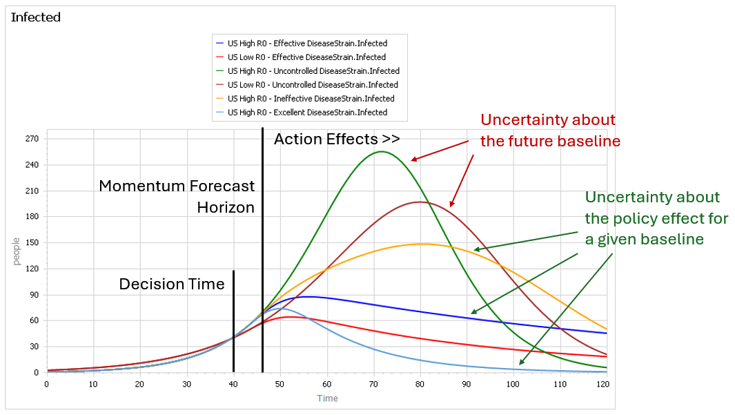
This is a set of scenarios from a simple SIR epidemic model in Ventity.
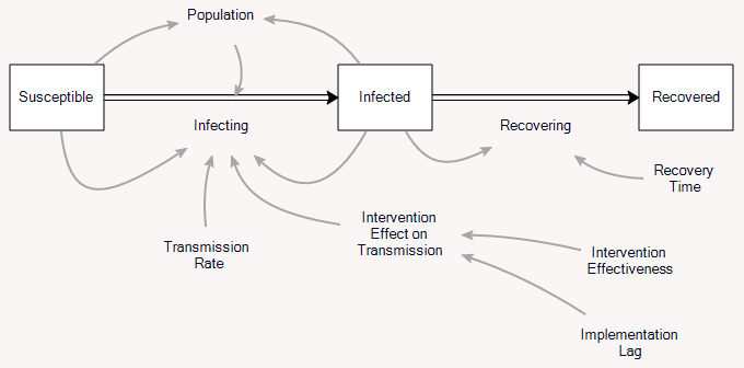
There are two sources of uncertainty in this model: the aggressiveness of the disease (transmission rate) and the effectiveness of an NPI policy that reduces transmission.
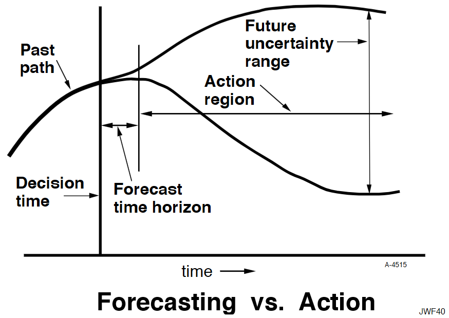
Early in the epidemic, at time 40 where the decision to intervene is made, it’s hard to tell the difference between a high transmission rate and a lower transmission rate with a slightly larger initial infected population. This is especially true in the real world, because early in an epidemic the information-gathering infrastructure is weak.
However, you can still make decent momentum forecasts by extrapolating from the early returns for a few more days – to time 45 or 50 perhaps. But this is not useful, because that roughly corresponds with the implementation lag for the policy. So, over the period of skilled momentum forecasts, it’s not possible to have much influence.
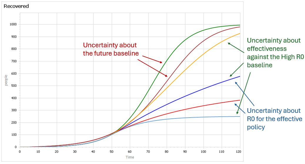
Beyond time 50, there’s a LOT of uncertainty in the disease trajectory, both from the uncontrolled baseline (is R0 low or high?) and the policy effectiveness (do masks work?). The yellow curve (high R0, low effectiveness) illustrates a key feature of epidemics: a policy that falls short of lowering the reproduction ratio below 1 results in continued growth of infection. It’s still beneficial, but constituents are likely to perceive this as a failure and abandon the policy (returning to the baseline, which is worse).
Some of these features are easier to see by looking at the cumulative outcome. Notice that the point prediction for times after about 60 has extremely large variance. But not everything is uncertain. In the uncontrolled baseline runs (green and brownish), eventually almost everyone gets the disease, it’s a matter of when not if, so uncertainty actually decreases after time 90 or so. Also, even though the absolute outcome varies a lot, the policy always improves on the baseline (at least neglecting cost, as we are here). So, while the forecast for time 100 might be bad, the contingent prediction for the effect of the policy is qualitatively insensitive to the uncertainty.