Tasty Menu

From the WPI online graduate program and courses in system dynamics:

Truly a fine lineup!

Model quality: the missing link

A number of developments are making model quality control increasingly crucial.

  • Models are generally playing a wider role in policy debates. Efforts like the Climate CoLab are making models accessible to wide audiences for interactive use.
  • The use of automated stochastic optimization and exploratory modeling and analysis (EMA) is likely to take models into parts of their parameter spaces that the modeler herself has not explored.
  • Standards like SMILE/XMILE will make models and model components more reusable and shareable.

I think this could all come to a bad end, in which priesthoods are paid to develop competing models that are incomprehensible to the general public, thus reducing modeling to a sophisticated form of propaganda.

Fortunately, some elements of an antidote to this dystopia are at hand, including documentation standards and tools and languages for expressing Reality Checks on model behavior. But I think we need a lot more. For example,

  • Standards could include metadata standards, so that model components are self-documenting in ways that make it possible for users to easily discover their limitations.
  • EMA tools could be directed towards discovery of model problems before policy analysis commences.
  • Tools that present models online could expose their innards as well as results.
  • Languages are needed for meta-reality checks, that describe and test higher level assumptions like perfect foresight (or lack thereof).

Perhaps most importantly, model quality needs to become a pervasive part of the culture of model building and consumption in all disciplines.

The Temperature-System Dynamics feedback

The recurrent heat waves coincident with system dynamics conferences have led me to some new insights about the co-evolution of systems thinking and climate. I’m hoping that I can get a last minute plenary slot for this blockbuster finding.

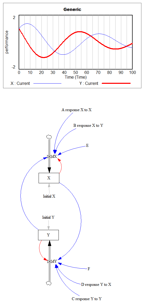
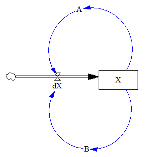
A priori, it should be obvious that temperature and system dynamics are linked. Here’s my dynamic hypothesis:

This hardly requires proof, but nevertheless data fully confirm the relationships.

Most obviously, the SD conference always occurs in July, the hottest month. The 2011 conference in Washington DC was the hottest July ever in that locale.

In addition, the timing of major works in SD coincides with warm years near Boston, the birthplace of the field.

I think we can consider this hypothesis definitively proven. All that remains is to put policies in place to ensure the continued health of SD, in order to prevent a global climatic catastrophe.


Do social negative feedbacks achieve smooth adjustment?

I’m rereading some of the history of global modeling, in preparation for the SD conference.

From Models of Doom, the Sussex critique of Limits to Growth:

Marie Jahoda, Chapter 14, Postscript on Social Change

The point is … to highlight a conception of man in world dynamics which seems to have led in all areas considered to an underestimation of negative feedback loops that bend the imaginary exponential growth curves to gentler slopes than “overshoot and collapse”. … Man’s fate is shaped not only by what happens to him but also by what he does, and he acts not just when faced with catastrophe but daily and continuously.

Meadows, Meadows, Randers & Behrens, A Response to Sussex:

The Sussex group confuses the numerical properties of our preliminary World models with the basic dynamic attributes of the world system described in the Limits to Growth. We suggest that exponential growth, physical limits, long adaptive delays, and inherent instability are obvious, general attributes of the present global system.

Who’s right?

I think we could all agree that the US housing market is vastly simpler than the world. It lies within a single political jurisdiction. Most of its value is private rather than a public good. It is fairly well observed, dense with negative feedbacks like price and supply/demand balance, and unfolds on a time scale that is meaningful to individuals. Delays like the pipeline of houses under construction are fairly salient. Do these benign properties “bend the imaginary exponential growth curves to gentler slopes than ‘overshoot and collapse'”?

Early warnings of catastrophe

There are warning signs when the active structure of a system is changing. But a new paper shows that they may not always be helpful for averting surprise catastrophes.

Catastrophic Collapse Can Occur without Early Warning: Examples of Silent Catastrophes in Structured Ecological Models (PLOS ONE – open access)

Catastrophic and sudden collapses of ecosystems are sometimes preceded by early warning signals that potentially could be used to predict and prevent a forthcoming catastrophe. Universality of these early warning signals has been proposed, but no formal proof has been provided. Here, we show that in relatively simple ecological models the most commonly used early warning signals for a catastrophic collapse can be silent. We underpin the mathematical reason for this phenomenon, which involves the direction of the eigenvectors of the system. Our results demonstrate that claims on the universality of early warning signals are not correct, and that catastrophic collapses can occur without prior warning. In order to correctly predict a collapse and determine whether early warning signals precede the collapse, detailed knowledge of the mathematical structure of the approaching bifurcation is necessary. Unfortunately, such knowledge is often only obtained after the collapse has already occurred.

To get the insight, it helps to back up a bit. (If you haven’t read my posts on bifurcations and 1D vector fields, they’re good background for this.)

Consider a first order system, with a flow that is a sinusoid, plus noise:

Flow=a*SIN(Stock*2*pi) + disturbance

For different values of a, and disturbance = 0, this looks like:

For a = 1, the system has a stable point at stock=0.5. The gain of the negative feedback that maintains the stable point at 0.5, given by the slope of the stock-flow phase plot, is strong, so the stock will quickly return to 0.5 if disturbed.

For a = -1, the system is unstable at 0.5, which has become a tipping point. It’s stable at the extremes where the stock is 0 or 1. If the stock starts at 0.5, the slightest disturbance triggers feedback to carry it to 0 or 1.

For a = 0.04, the system is approaching the transition (i.e. bifurcation) between stable and unstable behavior around 0.5. The gain of the negative feedback that maintains the stable point at 0.5, given by the slope of the stock-flow phase plot, is weak. If something disturbs the system away from 0.5, it will be slow to recover. The effective time constant of the system around 0.5, which is inversely proportional to a, becomes long for small a. This is termed critical slowing down.

For a=0 exactly, not shown, there is no feedback and the system is a pure random walk that integrates the disturbance.

The neat thing about critical slowing down, or more generally the approach of a bifurcation, is that it leaves fingerprints. Here’s a run of the system above, with a=1 (stable) initially, and ramping to a=-.33 (tipping) finally. It crosses a=0 (the bifurcation) at T=75. The disturbance is mild pink noise.

Notice that, as a approaches zero, particularly between T=50 and T=75, the variance of the stock increases considerably.

This means that you can potentially detect approaching bifurcations in time series without modeling the detailed interactions in the system, by observing the variance or similar, better other signs. Such analyses indicate that there has been a qualitative change in Arctic sea ice behavior, for example.

Now, back to the original paper.

It turns out that there’s a catch. Not all systems are neatly one dimensional (though they operate on low-dimensional manifolds surprisingly often).

In a multidimensional phase space, the symptoms of critical slowing down don’t necessarily reveal themselves in all variables. They have a preferred orientation in the phase space, associated with the eigenvectors of the eigenvalue that’s changing at the bifurcation.

The authors explore a third-order ecological model with juvenile and adult prey and a predator:

Predators undergo a collapse when their mortality rate exceeds a critical value (.553). Here, I vary the mortality rate gradually from .55 to .56, with the collapse occurring around time 450:

Note that the critical value of the mortality rate is actually passed around time 300, so it takes a while for the transient collapse to occur. Also notice that the variance of the adult population changes a lot post-collapse. This is another symptom of qualitative change in the dynamics.

The authors show that, in this system, approaching criticality of the predator mortality rate only reveals itself in increased variance or autocorrelation if noise impacts the juvenile population, and even then you have to be able to see the juvenile population.

We have shown three examples where catastrophic collapse can occur without prior early warning signals in autocorrelation or variance. Although critical slowing down is a universal property of fold bifurcations, this does not mean that the increased sensitivity will necessarily manifest itself in the system variables. Instead, whether the population numbers will display early warning will depend on the direction of the dominant eigenvector of the system, that is, the direction in which the system is destabilizing. This theoretical point also applies to other proposed early warning signals, such as skewness [18], spatial correlation [19], and conditional heteroscedasticity [20]. In our main example, early warning signal only occurs in the juvenile population, which in fact could easily be overlooked in ecological systems (e.g. exploited, marine fish stocks), as often only densities of older, more mature individuals are monitored. Furthermore, the early warning signals can in some cases be completely absent, depending on the direction of the perturbations to the system.

They then detail some additional reasons for lack of warning in similar systems.

In conclusion, we propose to reject the currently popular hypothesis that catastrophic shifts are preceded by universal early warning signals. We have provided counterexamples of silent catastrophes, and we have pointed out the underlying mathematical reason for the absence of early warning signals. In order to assess whether specific early warning signals will occur in a particular system, detailed knowledge of the underlying mathematical structure is necessary.

In other words, critical slowing down is a convenient, generic sign of impending change in a time series, but its absence is not a reliable indicator that all is well. Without some knowledge of the system in question, surprise can easily occur.

I think one could further strengthen the argument against early warning by looking at transients. In my simulation above, I’d argue that it takes at least 100 time units to detect a change in the variance of the juvenile population with any confidence, after it passes the critical point around T=300 (longer, if someone’s job depends on not seeing the change). The period of oscillations of the adult population in response to a disturbance is about 20 time units. So it seems likely that early warning, even where it exists, can only be established on time scales that are long with respect to the natural time scale of the system and environmental changes that affect it. Therefore, while signs of critical slowing down might exist in principle, they’re not particularly useful in this setting.

The models are in my library.

Catastrophic Collapse Can Occur without Early Warning: Examples of Silent Catastrophes in Structured Ecological Models

Causality in nonlinear systems

Sugihara et al. have a really interesting paper in Science, on detection of causality in nonlinear dynamic systems. It’s paywalled, so here’s an excerpt with some comments.

Abstract: Identifying causal networks is important for effective policy and management recommendations on climate, epidemiology, financial regulation, and much else. We introduce a method, based on nonlinear state space reconstruction, that can distinguish causality from correlation. It extends to nonseparable weakly connected dynamic systems (cases not covered by the current Granger causality paradigm). The approach is illustrated both by simple models (where, in contrast to the real world, we know the underlying equations/relations and so can check the validity of our method) and by application to real ecological systems, including the controversial sardine-anchovy-temperature problem.

Identifying causality in complex systems can be difficult. Contradictions arise in many scientific contexts where variables are positively coupled at some times but at other times appear unrelated or even negatively coupled depending on system state.

Although correlation is neither necessary nor sufficient to establish causation, it remains deeply ingrained in our heuristic thinking. … the use of correlation to infer causation is risky, especially as we come to recognize that nonlinear dynamics are ubiquitous. Continue reading “Causality in nonlinear systems”

Fun with 1D vector fields

Phase plots are the key to understanding life, the universe and the dynamics of everything.

Well, maybe that’s a bit of an overstatement. But they do nicely explain tipping points and bifurcations, which explain a heck of a lot (as I’ll eventually get to).

Fortunately, phase plots for simple systems are easy to work with. Consider a one-dimensional (first-order) system, like the stock and flow in my bathtub posts.

stock & flow

In Vensim lingo, you’d write this out as,

Stock = INTEG( Flow, Initial Stock )
Flow = ... {some function of the Stock and maybe other stuff}

In typical mathematical notation, you might write it as a differential equation, like

x' = f(x)

where x is the stock and x’ (dx/dt) is the flow.

This system (or vector field) has a one dimensional phase space – i.e. a line – because you can completely characterize the state of the system by the value of its single stock.

Fortunately, paper is two dimensional, so we can use the second dimension to juxtapose the flow with the stock (x’ with x), producing a phase plot that helps us get some intuition into the behavior of this stock-flow system. Here’s an example:

Pure accumulation

In this case, the flow is always above the x-axis, i.e. always positive, so the stock can only go up. The flow is constant, irrespective of the stock level, so there’s no feedback and the stock’s slope is constant.

Left: flow vs. stock. Right: resulting behavior of the stock over time.

Exponential growth

Adding feedback makes things more interesting.

In this simplest-possible first order positive feedback loop, the flow is proportional to the stock, so the stock-flow relationship is a rising line (left frame). There’s a trivial equilibrium (or fixed point) at stock = flow = 0, but it’s unstable, so it’s indicated with a hollow circle. An arrowhead indicates the direction of motion in the phase plot.

The resulting behavior is exponential growth (right frame). The bigger the stock gets, the steeper its slope gets.

Exponential decay

Negative feedback just inverts this case. The flow is below 0 when the stock is positive, and the system moves toward the origin instead of away from it.

The equilibrium at 0 is now stable, so it has a solid circle.

Linear systems like those above can have only one equilibrium. Geometrically, this is because the line of stock-flow proportionality can only cross 0 (the x axis) once. Mathematically, it’s because a system with a single state can have only one eigenvalue/eigenvector pair. Things get more interesting when the system is nonlinear.

S-shaped (logistic) growth

Here, the flow crosses zero twice, so there are two fixed points. The one at 0 is unstable, so as long as the stock is initially >0, it will rise to the stable equilibrium at 1.

(Note that there’s no reason to constrain the axes to the 0-1 unit line; it’s just a graphical convenience here.)

Tipping point

A phase diagram for a nonlinear model can have as many zero-crossings as you like. My forest cover toy model has five. A system can then have multiple equilibria. A pair of stable equilibria bracketing an unstable equilibrium creates a tipping point.

In this arrangement, the stable fixed points at 0 and 1 constitute basins of attraction that draw in any trajectories of the stock that lie in their half of the unit line. The unstable point at 0.5 is the fence between the basins, i.e. the tipping point. Any trajectory starting with the stock near 0.5 is drawn to one of the extremes. While stock=0.5 is theoretically possible permanently, real systems always have noise that will trigger the runaway.

If the stock starts out near 1, it will stay there fairly robustly, because feedback will restore that state from any excursion. But if some intervention or noise pushes the stock below 0.5, feedback will then draw it toward 0. Once there, it will be fairly robustly stuck again. This behavior can be surprising and disturbing if 1=good and 0=bad.

This is the very thing that happens in project fire fighting, for example. The 64 trillion dollar question is whether tipping point dynamics create perilous boundaries in the earth system, e.g., climate.

Not all systems are quite this simple. In particular, a stock is often associated with multiple flows. But it’s often helpful to look at first order subsystems of complex models in this way. For example, Jeroen Struben and John Sterman make good use of the phase plot to explore the dynamics of willingness (W) to purchase alternative fuel vehicles. They decompose the net flow of W (red) into multiple components that create a tipping point:

You can look at higher-order systems in the same way, though the pictures get messier (but prettier). You still preserve the attractive feature of this approach: by just looking at the topology of fixed points (or similar higher-dimensional sets), you can learn a lot about system behavior without doing any calculations.

What the heck is a bifurcation?

A while back, Bruce Skarin asked for an explanation of the bifurcations in a nuclear core model. I can’t explain that model well enough to be meaningful, but I thought it might be useful to explain the concept of bifurcations more generally.

A bifurcation is a change in the structure of a model that brings about a qualitative change in behavior. Qualitative doesn’t just mean big; it means different. So, a change in interest rates that bankrupts a country in a week instead of a century is not a bifurcation, because the behavior is exponential growth either way. A qualitative change in behavior is what we often talk about in system dynamics as a change in behavior mode, e.g. a change from exponential decay to oscillation.

This is closely related to differences in topology. In topology, the earth and a marble are qualitatively the same, because they’re both spheres. Scale doesn’t matter. A rugby ball and a basketball are also topologically the same, because you can deform one into the other without tearing.

On the other hand, you can’t deform a ball into a donut, because there’s no way to get the hole. So, a bifurcation on a ball is akin to pinching it until the sides meet, tearing out the middle, and stitching together the resulting edges. That’s qualitative.

Just as we can distinguish a ball from a donut from a pretzel by the arrangement of holes, we can recognize bifurcations by their effect on the arrangement of fixed points or other invariant sets in the state space of a system. Fixed points are just locations in state space at which the behavior of a system maps a point to itself – that is, they’re equilbria. More generally, an invariant set might be a an orbit (a limit cycle in two dimensions) or a chaotic attractor (in three).

A lot of parameter changes in a system will just move the fixed points around a bit, or deform them, without changing their number, type or relationship to each other. This changes the quantitative outcome, possibly by a lot, but it doesn’t change the qualitative behavior mode.

In a bifurcation, the population of fixed points and invariant sets actually changes. Fixed points can split into multiple points, change in stability, collide and annihilate one another, spawn orbits, and so on. Of course, for many of these things to exist or coexist, the system has to be nonlinear.

My favorite example is the supercritical pitchfork bifurcation. As a bifurcation parameter varies, a single stable fixed point (the handle of the pitchfork) abruptly splits into three (the tines): a pair of stable points, with an unstable point in the middle. This creates a tipping point: around the unstable fixed point, small changes in initial conditions cause the system to shoot off to one or the other stable fixed points.

Similarly, a Hopf bifurcation emerges when a fixed point changes in stability and a periodic orbit emerges around it. Periodic orbits often experience period doubling, in which the system takes two orbits to return to its initial state, and repeated period doubling is a route to chaos.

I’ve posted some model illustrating these and others here.

A bifurcation typically arises from a parameter change. You’ll often see diagrams that illustrate behavior or the location of fixed points with respect to some bifurcation parameter, which is just a model constant that’s varied over some range to reveal the qualitative changes. Some bifurcations need multiple coordinated changes to occur.

Of course, a constant parameter in one conception of a model might be an endogenous state in another – on a longer time horizon, for example. You can also think of a structure change (adding a feedback loop) as a parameter change, where the parameter is 0 (loop is off) or 1 (loop is on).

Bifurcations provide one intuitive explanation for the old SD contention that structure is more important than parameters. The structure of a system will often have a more significant effect on the kinds of fixed points or sets that can exist than the details of the parameters. (Of course, this is tricky, because it’s true, except when it’s not.  Sensitive parameters may exist, and in nonlinear systems, hard-to-find sensitive combinations may exist. Also, sensitivity may exist for reasons other than bifurcation.)

Why does this matter? For decision makers, it’s important because it’s easy to get comfortable with stable operation of a system in one regime, and then to be surprised when the rules suddenly change in response to some unnoticed or unmanaged change of state or parameters. For the nuclear reactor operator, stability is paramount, and it would be more than a little disturbing for limit cycles to emerge following a Hopf bifurcation induced by some change in operating parameters.

More on this later.

A project power law experiment

Taking my own advice, I grabbed a simple project model and did a Monte Carlo experiment to see if project performance had a heavy tailed distribution in response to normal and uniform inputs.

The model is the project tipping point model from Taylor, T. and Ford, D.N. Managing Tipping Point Dynamics in Complex Construction Projects ASCE Journal of Construction Engineering and Management. Vol. 134, No. 6, pp. 421-431. June, 2008, kindly supplied by David.

I made a few minor modifications to the model, to eliminate test inputs, and constructed a sensitivity input on a few parameters, similar to that described here. I used project completion time (the time at which 99% of work is done) as a performance metric. In this model, that’s perfectly correlated with cost, because the workforce is constant.

The core structure is the flow of tasks through the rework cycle to completion:

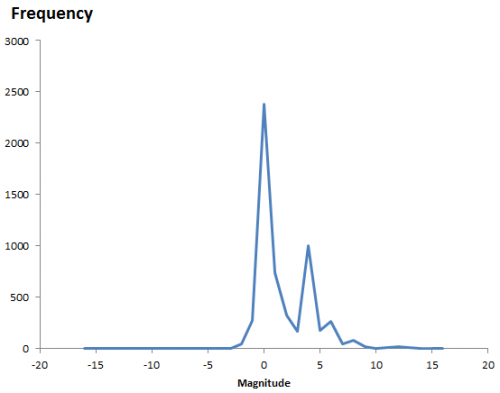
The initial results were baffling. The distribution of completion times was bimodal:

Worse, the bimodality didn’t appear to be correlated with any particular input:

Excerpt from a Weka scatterplot matrix of sensitivity inputs vs. log completion time.

Trying to understand these results with a purely black-box statistical approach is a hard road. The sensible thing is to actually look at the model to develop some insight into how the structure determines the behavior. So, I fired it up in Synthesim and did some exploration.

It turns out that there are (at least) two positive loops that cause projects to explode in this model. One is the rework cycle: work that is done wrong the first time has to be reworked – and it might be done wrong the second time, too. This is a positive loop with gain < 1, so the damage is bounded, but large if the error rate is high. A second, related loop is “ripple effects” – the collateral damage of rework.

My Monte Carlo experiment was, in some cases, pushing the model into a region with ripple+rework effects approaching 1, so that every task done creates an additional task. That causes the project to spiral into the right sub-distribution, where it is difficult or impossible to complete.

This is interesting, but more pathological than what I was interested in exploring. I moderated my parameter choices and eliminated a few test inputs in the model, and repeated the experiment.

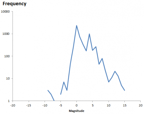
Voila:

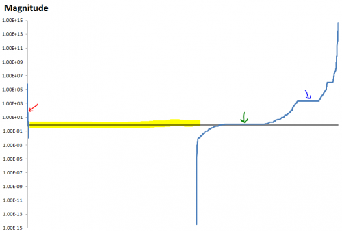
Normal+uniformly-distributed uncertainty in project estimation, productivity and ripple/rework effects generates a lognormal-ish left tail (parabolic on the log-log axes above) and a heavy Power Law right tail.*

The interesting thing about this is that conventional project estimation methods will completely miss it. There are no positive loops in the standard CPM/PERT/Gantt view of a project. This means that a team analyzing project uncertainty with Normal errors in will get Normal errors out, completely missing the potential for catastrophic Black Swans.

Continue reading “A project power law experiment”