The traditional picture of information sources for modeling is a funnel. For example, in Some Basic Concepts in System Dynamics (2009), Forrester showed:
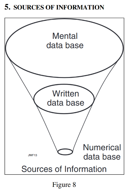 I think the diagram, or at least the concept, is much older than that.
However, I think the landscape has changed a lot, with more to come. Generally, the mental database hasn’t changed too much, but the numerical database has grown a lot. The funnel isn’t 1-dimensional, so the relationships have changed on some axes, but not so much on others.
Notionally, I’d propose that the situation is something like this:
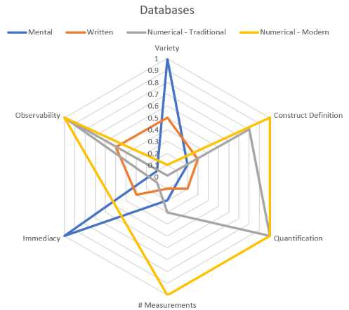
The mental database is still king for variety of concepts and immediacy or salience of information (especially to the owner of the brain involved). And, it still has some weaknesses, like the inability to easily observe, agree on and quantify the constructs included in it. In the last few decades, the numerical database has extended its reach tremendously.
The proper shape of the plot is probably very domain specific. When I drew this, I had in mind the typical corporate or policy setting, where information systems contain only a fraction of the information necessary to understand the organizations involved. But in some areas, the reverse may be true. For example, in earth systems, datasets are vast and include measurements that human senses can’t even make, whereas personal experience – and therefore mental models – is limited and treacherous.
I think I’ve understated the importance of the written database in the diagram above – perhaps I’m missing a dimension characterizing its cumulative nature (compared to the transience of mental databases). There’s also an interesting evolution underway, as tools for text analysis and large language models (ChatGPT) are making the written database more numerical in nature.
Finally, I think there’s a missing database in the traditional framework, which has growing importance. That’s the database of models themselves. They’ve been around for a long time – especially in physical sciences, but also corporate spreadsheets and the like. But increasingly, reasonably sophisticated models of organizational components are available as inputs to higher-level strategic problem solving modeling efforts.