A newish set of papers (1. Theory (preprint); 2. Applications (preprint); 3. Extension) is making the rounds on the climate skeptic sites, with – ironically – little skepticism applied.
The claim is bold:
… According to the commonly assumed causality link, increased [CO2] causes a rise in T. However, recent developments cast doubts on this assumption by showing that this relationship is of the hen-or-egg type, or even unidirectional but opposite in direction to the commonly assumed one. These developments include an advanced theoretical framework for testing causality based on the stochastic evaluation of a potentially causal link between two processes via the notion of the impulse response function. …. All evidence resulting from the analyses suggests a unidirectional, potentially causal link with T as the cause and [CO2] as the effect.
Galileo complex seeps in when the authors claim that absence of correlation or impulse response from CO2 -> temperature proves absence of causality:
Clearly, the results […] suggest a (mono-directional) potentially causal system with T as the cause and [CO2] as the effect. Hence the common perception that increasing [CO2] causes increased T can be excluded as it violates the necessary condition for this causality direction.
Unfortunately, these claims are bogus. Here’s why.
The authors estimate impulse response functions between CO2 and temperature (and back), using the following formalism:
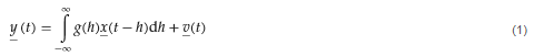
where g(h) is the response at lag h. As the authors point out, if
the IRF is zero for every lag except for the specific lag ℎ0, then Equation (1) becomes y(t)=bx(t-h0) +v(t). This special case is equivalent to simply correlating y(t) with x(t-h0) at any time instance . It is easy to find (cf. linear regression) that in this case the multiplicative constant is the correlation coefficient of y(t) and x(t-h0) multiplied by the ratio of the standard deviations of the two processes.
Now … anyone who claims to have an “advanced theoretical framework for testing causality” should be aware of the limitations of linear regression. There are several possible issues that might lead to misleading conclusions about causality.
Problem #1 here is bathtub statistics. Temperature integrates the radiative forcing from CO2 (and other things). This is not debatable – it’s physics. It’s old physics, and it’s experimental, not observational. If you question the existence of the effect, you’re basically questioning everything back to the Enlightenment. The implication is that no correlation is expected between CO2 and temperature, because integration breaks pattern matching. The authors purport to avoid integration by using first differences of temperature and CO2. But differencing both sides of the equation doesn’t solve the integration problem; it just kicks the can down the road. If y integrates x, then patterns of the integrals or derivatives of y and x won’t match either. Even worse differencing filters out the signals of interest.
Problem #2 is that the model above assumes only equation error (the term v(t) on the right hand side). In most situations, especially dynamic systems, both the “independent” (a misnomer) and dependent variables are subject to measurement error, and this dilutes the correlation or slope of the regression line (aka attenuation bias), and therefore also the IRF in the authors’ framework. In the case of temperature, the problem is particularly acute, because temperature also integrates internal variability of the climate system (weather) and some of this variability is autocorrelated on long time scales (because for example oceans have long time constants). That means the effective number of data points is a lot less than the 60 years or 720 months you’d expect from simple counting.
Dynamic variables are subject to other pathologies, generally under the heading of endogeneity bias, and related features with similar effects like omitted variable bias. Generalizing the approach to distributed lags in no way mitigates these. The bottom line is that absence of correlation doesn’t prove absence of causation.
Admittedly, even Nobel Prize winners can screw up claims about causality and correlation and estimate dynamic models with inappropriate methods. But causality confusion isn’t really a good way to get into that rarefied company.
I think methods purporting to assess causality exclusively from data are treacherous in general. The authors’ proposed method is provably wrong in some cases, including this one, as is Granger Causality. Even if you have pretty good assumptions, you’ll always find a system that violates them. That’s why it’s so important to take data-driven results with a grain of salt, and look for experimental control (where you can get it) and mechanistic explanations.
One way to tell if you’ve gotten causality wrong is when you “discover” mechanisms that are physically absurd. That happens on a spectacular scale in the third paper:
… we find Δ=23.5 and 8.1 Gt C/year, respectively, i.e., a total global increase in the respiration rate of Δ=31.6 Gt C/year. This rate, which is a result of natural processes, is 3.4 times greater than the CO2 emission by fossil fuel combustion (9.4 Gt C /year including cement production).
To put that in perspective, the authors propose a respiration flow that would put the biosphere about 30% out of balance. This implies a mass flow of trees harvested, soils destroyed, etc. 3.4 times as large as the planetary flow of fossil fuels. That would be about 4 cubic kilometers of wood, for example. In the face of the massive outflow from the biosphere, the 9.4 GtC/yr from fossil fuels went where, exactly? Extraordinary claims require extraordinary evidence, but the authors apparently haven’t pondered how these massive novel flows could be squared with other lines of evidence, like C isotopes, ocean Ph, satellite CO2, and direct estimates of land use emissions.
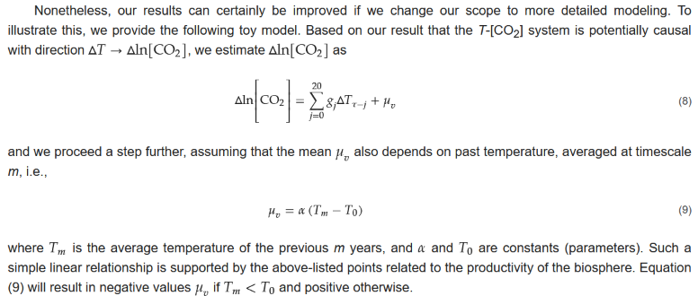
This “insight” is used to construct a model of the temperature->CO2 process:
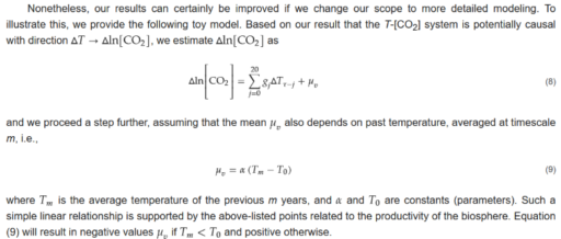
In this model, the trend in CO2 is explained almost exclusively by the mean temperature effect mu_v = alpha*(T-T0). That effect is entirely ad hoc, with no basis in the impulse response framework.
How do we get into this pickle? I think the simple answer is that the authors’ specification of the system is incomplete. As above, they define a causal system,
y(t) = ∫g1(h)x(t-h)dh
x(t) = ∫g2(h)y(t-h)dh
where g(.) is an impulse response function weighting lags h and the integral is over h from 0 to infinity (because only nonnegative lags are causal). In their implementation, x and y are first differences, so in their climate example, Δlog(CO2) and ΔTemp. In the estimation of the impulse lag structures g(.), the authors impose nonnegativity and (optionally) smoothness constraints.
A more complete specification is roughly:
Y = A*X + U
dX/dt = B*X + E
where
- X is a vector of system states (e.g., CO2 and temperature)
- Y is a vector of measurements (observed CO2 and temperature)
- A and B are matrices of coefficients (this is a linear view of the system, but could easily be generalized to nonlinear functions)
- E is driving noise perturbing the state, and therefore integrated into it
- U is measurement error
My notation could be improved to consider covariance and state-dependent noise, though it’s not really necessary here. Fred Schweppe wrote all this out decades ago in Uncertain Dynamic Systems, and you can now find it in many texts like Stengel’s Optimal Control and Estimation. Dixit and Pindyck transplanted it to economics and David Peterson brought it to SD where it found its way into Vensim as the combination of Kalman filtering and optimization.
How does this avoid the pitfalls of the Koutsoyiannis et al. approach?
- An element of X can integrate any other element of X, including itself.
- There are no arbitrary restrictions (like nonnegativity) on the impulse response function.
- The system model (A, B, and any nonlinear elements augmenting the framework) can incorporate a priori structural knowledge (e.g., physics).
- Driving noise and measurement error are recognized and can be estimated along with everything else.
Does the difference matter? I’ll leave that for a second post with some examples.

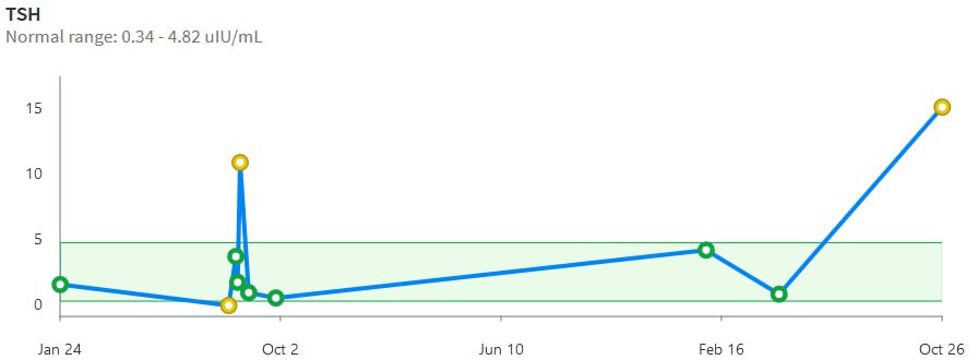
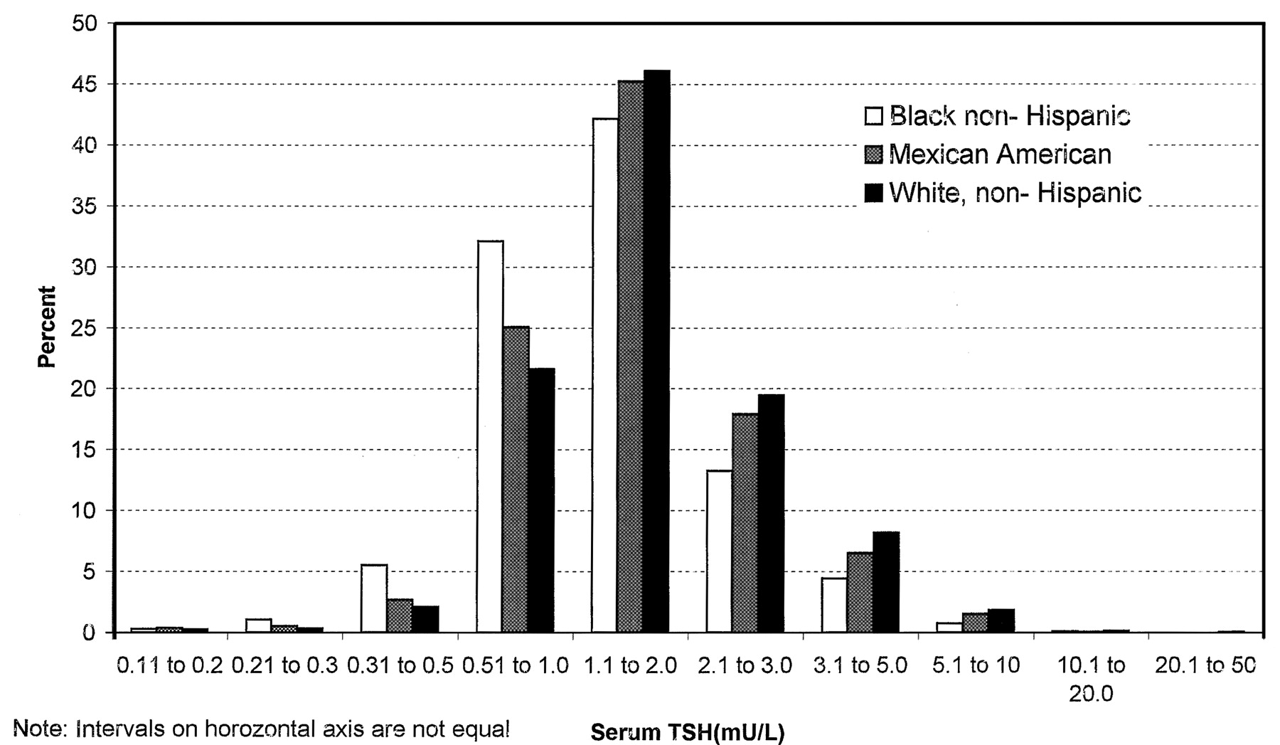
 It’s actually not as bad as you’d think: the irregular axis is actually a decent approximation of a log-linear scale:
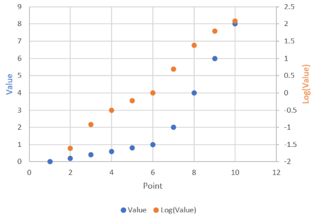 My main gripe is that the perceptual midpoint of the ATA range bar on the chart is roughly 0.9, whereas the true logarithmic midpoint is more like 1.6. The NACB bar is similarly distorted.