One of the smaller and cuter stakeholders in climate change is the pika, an alpine mini-rabbit that has nowhere to go as warming takes their habitable zone above mountaintops.
Support pika research on RocketHub.
Don't just do something, stand there! Reflections on the counterintuitive behavior of complex systems, seen through the eyes of System Dynamics, Systems Thinking and simulation.
One of the smaller and cuter stakeholders in climate change is the pika, an alpine mini-rabbit that has nowhere to go as warming takes their habitable zone above mountaintops.
Support pika research on RocketHub.
Roy Spencer on reducing emissions by increasing emissions:
COL: Let’s say tomorrow, evidence is found that proves to everyone that global warming as a result of human released emissions of CO2 and methane, is real. What would you suggest we do?
SPENCER: I would say we need to grow the economy as fast as possible, in order to afford the extra R&D necessary to develop new energy technologies. Current solar and wind technologies are too expensive, unreliable, and can only replace a small fraction of our energy needs. Since the economy runs on inexpensive energy, in order to grow the economy we will need to use fossil fuels to create that extra wealth. In other words, we will need to burn even more fossil fuels in order to find replacements for fossil fuels.
On the face of it, this is absurd. Reverse a positive feedback loop by making it stronger? But it could work, if given the right structure – a relative quit smoking by going in a closet to smoke until he couldn’t stand it anymore. Here’s what I can make of the mental model:
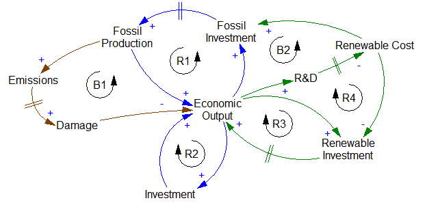 Spencer’s arguing that we need to run reinforcing loops R1 and R2 as hard as possible, because loop R3 is too weak to sustain the economy, because renewables (or more generally non-emitting sources) are too expensive. R1 and R2 provide the wealth to drive R&D, in a virtuous cycle R4 that activates R3 and shuts down the fossil sector via B2. There are a number of problems with this thinking.
In truth, these feedbacks are already present in many energy models. Most of those are standard economic stuff – equilibrium, rational expectations, etc. – assumptions which favor growth. Yet among the subset that includes endogenous technology, I’m not aware of a single instance that finds a growth+R&D led policy to be optimal or even effective.
It’s time for the techno-optimists like Spencer and Breakthrough to put up or shut up. Either articulate the argument in a formal model that can be shared and tested, or admit that it’s a nice twinkle in the eye that regrettably lacks evidence.
The Reinhart & Rogoff debt/growth paper continues to make a stir for it’s basic Excel errors. Colbert has the latest & funniest take on it.
Two things about this surprise me.
Confronted with obvious and irrefutable errors, the authors double down and admit nothing. They also downplay the significance of the results, ‘… we are very careful in all our papers to speak of “association” and not “causality” …’
But of course the (amplified) message, Debt/GDP>90%=doom, was taken causally in the policy world; see the multiple clips in the intro to the Colbert video. Politicians are nuts to accord one paper in a sea of macroeconomic thought so much weight, but I guess this was the one they liked.
It’s time* for environmentalists (and everyone else) to give up on a myriad of second-best regulatory policies and push for a simple emissions price (i.e. a carbon tax). The latest reason: green subsidies are unraveling under adverse energy market conditions. There are many others:
All of the above have some role to play, but without prices as a keystone economic signal, they’re fighting the tide. Moreover, together they have a large cost in administrative complexity, which gives opponents a legitimate reason to whine about bureaucracy and promotes regulatory capture.
If all the effort that’s now expended in fragmented venues to create these policies were focused on one measure, would it be enough to pass a significant emissions price with fair revenue recycling and a border adjustment? I don’t know for sure, but I’d like to see us try.
* Actually, I think it was time for a carbon tax at least 20 years ago.
Sugihara et al. have a really interesting paper in Science, on detection of causality in nonlinear dynamic systems. It’s paywalled, so here’s an excerpt with some comments.
Abstract: Identifying causal networks is important for effective policy and management recommendations on climate, epidemiology, financial regulation, and much else. We introduce a method, based on nonlinear state space reconstruction, that can distinguish causality from correlation. It extends to nonseparable weakly connected dynamic systems (cases not covered by the current Granger causality paradigm). The approach is illustrated both by simple models (where, in contrast to the real world, we know the underlying equations/relations and so can check the validity of our method) and by application to real ecological systems, including the controversial sardine-anchovy-temperature problem.
Identifying causality in complex systems can be difficult. Contradictions arise in many scientific contexts where variables are positively coupled at some times but at other times appear unrelated or even negatively coupled depending on system state.
…
Although correlation is neither necessary nor sufficient to establish causation, it remains deeply ingrained in our heuristic thinking. … the use of correlation to infer causation is risky, especially as we come to recognize that nonlinear dynamics are ubiquitous. Continue reading “Causality in nonlinear systems”
The EU declined backloading, a deferral of permit auctions that would have supported prices in the Emissions Trading System (ETS).
This is described imminent collapse to the system, threatening the achievement of emissions targets. Perhaps a political collapse is imminent – not my department – but the idea that low emissions prices threaten the system is a bit odd. The ETS price is a feedback mechanism. Low prices are a symptom, indicating that the marginal cost of meeting targets is extremely low. That should be a cause for celebration (except for traders).
For the umpteenth time, this shows the difficulty of running a system that invites wrangling over allocation and propagates noise from the economy into a market.
Meanwhile, carbon taxes grind away at their job.
Phase plots are the key to understanding life, the universe and the dynamics of everything.
Well, maybe that’s a bit of an overstatement. But they do nicely explain tipping points and bifurcations, which explain a heck of a lot (as I’ll eventually get to).
Fortunately, phase plots for simple systems are easy to work with. Consider a one-dimensional (first-order) system, like the stock and flow in my bathtub posts.
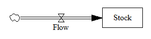
In Vensim lingo, you’d write this out as,
Stock = INTEG( Flow, Initial Stock )
Flow = ... {some function of the Stock and maybe other stuff}
In typical mathematical notation, you might write it as a differential equation, like
x' = f(x)
where x is the stock and x’ (dx/dt) is the flow.
This system (or vector field) has a one dimensional phase space – i.e. a line – because you can completely characterize the state of the system by the value of its single stock.
Fortunately, paper is two dimensional, so we can use the second dimension to juxtapose the flow with the stock (x’ with x), producing a phase plot that helps us get some intuition into the behavior of this stock-flow system. Here’s an example:
Pure accumulation
In this case, the flow is always above the x-axis, i.e. always positive, so the stock can only go up. The flow is constant, irrespective of the stock level, so there’s no feedback and the stock’s slope is constant.
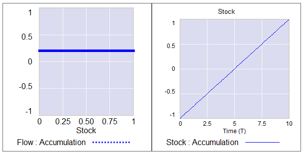 Left: flow vs. stock. Right: resulting behavior of the stock over time.
Exponential growth
Adding feedback makes things more interesting.
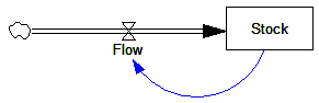
In this simplest-possible first order positive feedback loop, the flow is proportional to the stock, so the stock-flow relationship is a rising line (left frame). There’s a trivial equilibrium (or fixed point) at stock = flow = 0, but it’s unstable, so it’s indicated with a hollow circle. An arrowhead indicates the direction of motion in the phase plot.
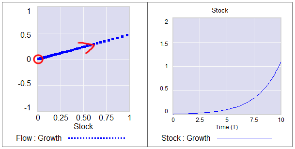
The resulting behavior is exponential growth (right frame). The bigger the stock gets, the steeper its slope gets.
Exponential decay
Negative feedback just inverts this case. The flow is below 0 when the stock is positive, and the system moves toward the origin instead of away from it.
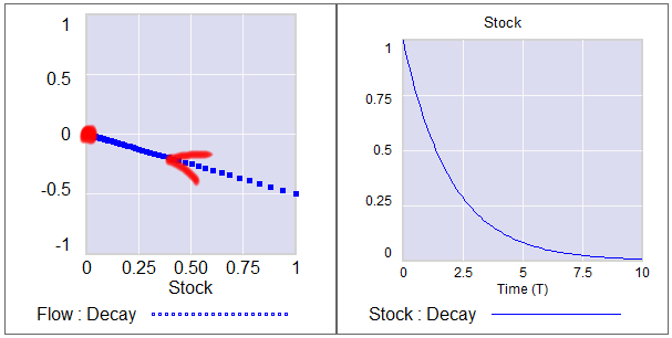 The equilibrium at 0 is now stable, so it has a solid circle.
Linear systems like those above can have only one equilibrium. Geometrically, this is because the line of stock-flow proportionality can only cross 0 (the x axis) once. Mathematically, it’s because a system with a single state can have only one eigenvalue/eigenvector pair. Things get more interesting when the system is nonlinear.
S-shaped (logistic) growth
Here, the flow crosses zero twice, so there are two fixed points. The one at 0 is unstable, so as long as the stock is initially >0, it will rise to the stable equilibrium at 1.
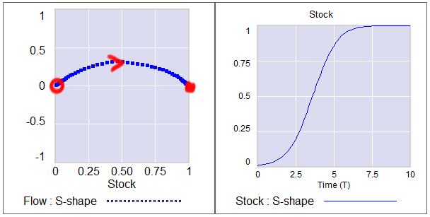 (Note that there’s no reason to constrain the axes to the 0-1 unit line; it’s just a graphical convenience here.)
A phase diagram for a nonlinear model can have as many zero-crossings as you like. My forest cover toy model has five. A system can then have multiple equilibria. A pair of stable equilibria bracketing an unstable equilibrium creates a tipping point.
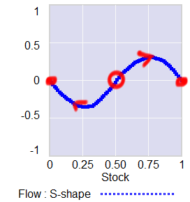 In this arrangement, the stable fixed points at 0 and 1 constitute basins of attraction that draw in any trajectories of the stock that lie in their half of the unit line. The unstable point at 0.5 is the fence between the basins, i.e. the tipping point. Any trajectory starting with the stock near 0.5 is drawn to one of the extremes. While stock=0.5 is theoretically possible permanently, real systems always have noise that will trigger the runaway.
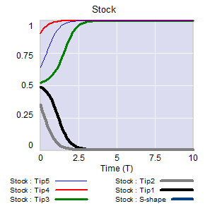 If the stock starts out near 1, it will stay there fairly robustly, because feedback will restore that state from any excursion. But if some intervention or noise pushes the stock below 0.5, feedback will then draw it toward 0. Once there, it will be fairly robustly stuck again. This behavior can be surprising and disturbing if 1=good and 0=bad.
This is the very thing that happens in project fire fighting, for example. The 64 trillion dollar question is whether tipping point dynamics create perilous boundaries in the earth system, e.g., climate.
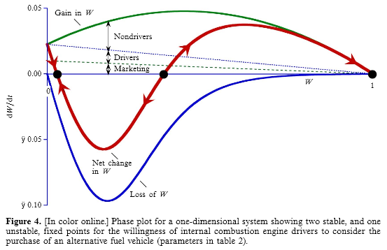
Not all systems are quite this simple. In particular, a stock is often associated with multiple flows. But it’s often helpful to look at first order subsystems of complex models in this way. For example, Jeroen Struben and John Sterman make good use of the phase plot to explore the dynamics of willingness (W) to purchase alternative fuel vehicles. They decompose the net flow of W (red) into multiple components that create a tipping point:
You can look at higher-order systems in the same way, though the pictures get messier (but prettier). You still preserve the attractive feature of this approach: by just looking at the topology of fixed points (or similar higher-dimensional sets), you can learn a lot about system behavior without doing any calculations.
File under “this would be funny if it weren’t frightening.”
HOUSE BILL No. 2366
By Committee on Energy and Environment
(a) No public funds may be used, either directly or indirectly, to promote, support, mandate, require, order, incentivize, advocate, plan for, participate in or implement sustainable development.
(2) “sustainable development” means a mode of human development in which resource use aims to meet human needs while preserving the environment so that these needs can be met not only in the present, but also for generations to come, but not to include the idea, principle or practice of conservation or conservationism.
Surely it’s not the “resource use aims to meet human needs” part that the authors find objectionable, so it must be the “preserving the environment so that these needs can be met … for generations to come” that they reject. The courts are going to have a ball developing a legal test separating that from conservation. I guess they’ll have to draw a line that distinguishes “present” from “generations to come” and declares that conservation is for something other than the future. Presumably this means that Kansas must immediately abandon all environment and resource projects with a payback time of more than a year or so.
But why stop with environment and resource projects? Kansas could simply set its discount rate for public projects to 100%, thereby terminating all but the most “present” of its investments in infrastructure, education, R&D and other power grabs by generations to come.
Another amusing contradiction:
(b) Nothing in this section shall be construed to prohibit the use of public funds outside the context of sustainable development: (1) For planning the use, development or extension of public services or resources; (2) to support, promote, advocate for, plan for, enforce, use, teach, participate in or implement the ideas, principles or practices of planning, conservation, conservationism, fiscal responsibility, free market capitalism, limited government, federalism, national and state sovereignty, individual freedom and liberty, individual responsibility or the protection of personal property rights;
So, what happens if Kansas decides to pursue conservation the libertarian way, by allocating resource property rights to create markets that are now missing? Is that sustainable development, or promotion of free market capitalism? More fun for the courts.
Perhaps this is all just a misguided attempt to make the Montana legislature look sane by comparison.
h/t Bloomberg via George Richardson
A while back, Bruce Skarin asked for an explanation of the bifurcations in a nuclear core model. I can’t explain that model well enough to be meaningful, but I thought it might be useful to explain the concept of bifurcations more generally.
A bifurcation is a change in the structure of a model that brings about a qualitative change in behavior. Qualitative doesn’t just mean big; it means different. So, a change in interest rates that bankrupts a country in a week instead of a century is not a bifurcation, because the behavior is exponential growth either way. A qualitative change in behavior is what we often talk about in system dynamics as a change in behavior mode, e.g. a change from exponential decay to oscillation.
This is closely related to differences in topology. In topology, the earth and a marble are qualitatively the same, because they’re both spheres. Scale doesn’t matter. A rugby ball and a basketball are also topologically the same, because you can deform one into the other without tearing.
On the other hand, you can’t deform a ball into a donut, because there’s no way to get the hole. So, a bifurcation on a ball is akin to pinching it until the sides meet, tearing out the middle, and stitching together the resulting edges. That’s qualitative.
Just as we can distinguish a ball from a donut from a pretzel by the arrangement of holes, we can recognize bifurcations by their effect on the arrangement of fixed points or other invariant sets in the state space of a system. Fixed points are just locations in state space at which the behavior of a system maps a point to itself – that is, they’re equilbria. More generally, an invariant set might be a an orbit (a limit cycle in two dimensions) or a chaotic attractor (in three).
A lot of parameter changes in a system will just move the fixed points around a bit, or deform them, without changing their number, type or relationship to each other. This changes the quantitative outcome, possibly by a lot, but it doesn’t change the qualitative behavior mode.
In a bifurcation, the population of fixed points and invariant sets actually changes. Fixed points can split into multiple points, change in stability, collide and annihilate one another, spawn orbits, and so on. Of course, for many of these things to exist or coexist, the system has to be nonlinear.
My favorite example is the supercritical pitchfork bifurcation. As a bifurcation parameter varies, a single stable fixed point (the handle of the pitchfork) abruptly splits into three (the tines): a pair of stable points, with an unstable point in the middle. This creates a tipping point: around the unstable fixed point, small changes in initial conditions cause the system to shoot off to one or the other stable fixed points.
Similarly, a Hopf bifurcation emerges when a fixed point changes in stability and a periodic orbit emerges around it. Periodic orbits often experience period doubling, in which the system takes two orbits to return to its initial state, and repeated period doubling is a route to chaos.
I’ve posted some model illustrating these and others here.
A bifurcation typically arises from a parameter change. You’ll often see diagrams that illustrate behavior or the location of fixed points with respect to some bifurcation parameter, which is just a model constant that’s varied over some range to reveal the qualitative changes. Some bifurcations need multiple coordinated changes to occur.
Of course, a constant parameter in one conception of a model might be an endogenous state in another – on a longer time horizon, for example. You can also think of a structure change (adding a feedback loop) as a parameter change, where the parameter is 0 (loop is off) or 1 (loop is on).
Bifurcations provide one intuitive explanation for the old SD contention that structure is more important than parameters. The structure of a system will often have a more significant effect on the kinds of fixed points or sets that can exist than the details of the parameters. (Of course, this is tricky, because it’s true, except when it’s not. Sensitive parameters may exist, and in nonlinear systems, hard-to-find sensitive combinations may exist. Also, sensitivity may exist for reasons other than bifurcation.)
Why does this matter? For decision makers, it’s important because it’s easy to get comfortable with stable operation of a system in one regime, and then to be surprised when the rules suddenly change in response to some unnoticed or unmanaged change of state or parameters. For the nuclear reactor operator, stability is paramount, and it would be more than a little disturbing for limit cycles to emerge following a Hopf bifurcation induced by some change in operating parameters.
Taking my own advice, I grabbed a simple project model and did a Monte Carlo experiment to see if project performance had a heavy tailed distribution in response to normal and uniform inputs.
The model is the project tipping point model from Taylor, T. and Ford, D.N. Managing Tipping Point Dynamics in Complex Construction Projects ASCE Journal of Construction Engineering and Management. Vol. 134, No. 6, pp. 421-431. June, 2008, kindly supplied by David.
I made a few minor modifications to the model, to eliminate test inputs, and constructed a sensitivity input on a few parameters, similar to that described here. I used project completion time (the time at which 99% of work is done) as a performance metric. In this model, that’s perfectly correlated with cost, because the workforce is constant.
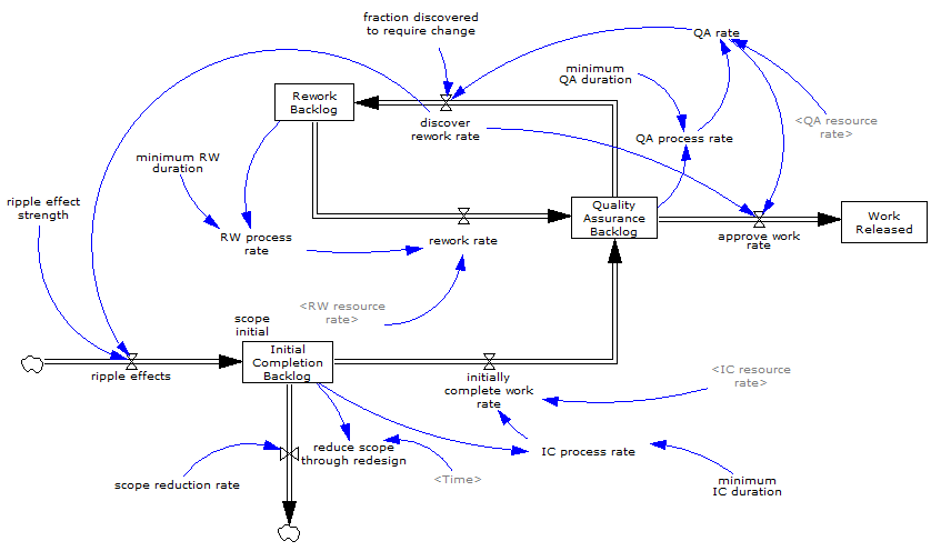
The core structure is the flow of tasks through the rework cycle to completion:
The initial results were baffling. The distribution of completion times was bimodal:
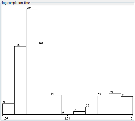
Worse, the bimodality didn’t appear to be correlated with any particular input:

Excerpt from a Weka scatterplot matrix of sensitivity inputs vs. log completion time.
Trying to understand these results with a purely black-box statistical approach is a hard road. The sensible thing is to actually look at the model to develop some insight into how the structure determines the behavior. So, I fired it up in Synthesim and did some exploration.
It turns out that there are (at least) two positive loops that cause projects to explode in this model. One is the rework cycle: work that is done wrong the first time has to be reworked – and it might be done wrong the second time, too. This is a positive loop with gain < 1, so the damage is bounded, but large if the error rate is high. A second, related loop is “ripple effects” – the collateral damage of rework.
My Monte Carlo experiment was, in some cases, pushing the model into a region with ripple+rework effects approaching 1, so that every task done creates an additional task. That causes the project to spiral into the right sub-distribution, where it is difficult or impossible to complete.
This is interesting, but more pathological than what I was interested in exploring. I moderated my parameter choices and eliminated a few test inputs in the model, and repeated the experiment.
Voila:
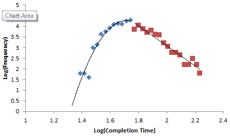 Normal+uniformly-distributed uncertainty in project estimation, productivity and ripple/rework effects generates a lognormal-ish left tail (parabolic on the log-log axes above) and a heavy Power Law right tail.*
The interesting thing about this is that conventional project estimation methods will completely miss it. There are no positive loops in the standard CPM/PERT/Gantt view of a project. This means that a team analyzing project uncertainty with Normal errors in will get Normal errors out, completely missing the potential for catastrophic Black Swans.