Climate Interactive has the story.
Try it yourself, or see it in action in an interactive webinar on June 3rd.

Don't just do something, stand there! Reflections on the counterintuitive behavior of complex systems, seen through the eyes of System Dynamics, Systems Thinking and simulation.
Climate Interactive has the story.
Try it yourself, or see it in action in an interactive webinar on June 3rd.
Yesterday’s news:
BONN, Germany (Reuters) – China, India and other developing nations joined forces on Wednesday to urge rich countries to make far deeper cuts in greenhouse gas emissions than planned by 2020 to slow global warming.
I’m sure that the mental model behind this runs something like, “the developed world created most of the problem up to this point, and they’re rich, so they should get busy making deep cuts, while we grow a little more to catch up.” Regardless of fairness considerations, that approach ignores the physics of the situation. If developing countries continue to increase emissions, it hardly matters how deep cuts are in the rich world. Either everyone plays along, or mitigation doesn’t work.
I fired up C-ROADS and ran a few scenarios to illustrate:
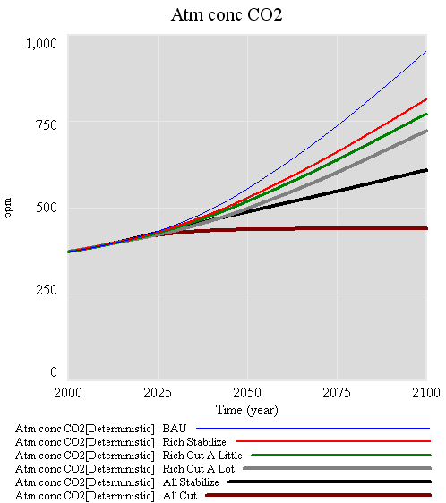
The top blue line is the AIFI business-as-usual, with rapid emissions growth. If rich nations stabilize emissions as of today, you get the red line – still much more than 2x CO2 at the end of the century. Whether the rich start cutting emissions a little (1%/yr, green) or a lot (5%/yr, green) after that makes relatively little difference, because emissions from the rich world quickly become a small share of the total. Getting everyone to merely stabilize emissions (at 2009 levels for the rich, 2020 for developing countries, black) makes a substantially bigger difference than deep cuts by the rich alone. Stabilizing CO2 in the atmosphere at a low level requires deep cuts by everyone (here 4%/year, brown).
If we’re serious about stabilization, it doesn’t make sense for the rich to decarbonize faster, so that the developing world can construct more carbon-dependent capital that will ultimately have to be deconstructed. It may sound “fair” in carbon-per-capita terms, but I don’t think that’s a very good measure of human welfare, and it’s unlikely to end up with a fair distribution of damages.
If the developing countries are really concerned about climate impacts (as they should be), they should be looking to the rich world for help getting onto a low-carbon path today, not in 20 years. They should also be willing to impose a carbon price on themselves. It won’t collapse their economies any more than it will ours. Without a price on carbon, rebound effects and leakage will eat up most gains, as the private sector responds to the real signal: “go green (but the price of carbon is zero, wink wink nudge nudge).” Their request to the rich should be about the transfers, property rights, and other changes it takes to get the job done with some measure of distributional fairness (a topic that won’t be popular in some circles).
Beth Sawin just presented our C-ROADS work in Copenhagen. The model will soon be available online and in other forms, for decision support and educational purposes. It helps people to understand the basic dynamics of the carbon cycle and climate, and to add up diverse regional proposals for emissions reductions, to see what they imply for the globe. It’s a small model, yet there are those who love it. No model can do everything, so I thought I’d point out a few other tools that are available online, fairly easy to use, and serve similar purposes.
From MNP, Netherlands. Like C-ROADS, runs interactively. The downloadable demo version is quite sophisticated, but emphasizes discovery of emissions trajectories that meet goals and constraints, rather than characterization of proposals on the table. The full research version, with sector/fuel detail and marginal abatement costs, is available on a case-by-case basis. Backed up by some excellent publications.
Ben Matthews’ Java Climate Model. Another interactive tool. Generates visually stunning output in realtime, which is remarkable given the scale and sophistication of the underlying model. Very rich; it helps to know what you’re after when you start to get into the deeper levels.
The tool used in AR4 to summarize the behavior of 19 GCMs, facilitating more rapid scenario experimentation and sensitivity analysis. Its companion SCENGEN does nice regional maps, which I haven’t really explored. MAGICC takes a few seconds to run, and while it has a GUI, detailed input and output is buried in text files, so I’m stretching the term “friendly” here.
I think these are the premier accessible tools out there, but I’m sure I’ve forgotten a few, so I’ll violate my normal editing rules and update this post as needed.
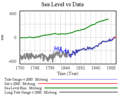
The pretty pictures look rather compelling, but we’re not quite done. A little QC is needed on the results. It turns out that there’s trouble in paradise:
#1 is not really a surprise; G discusses the sea level error structure at length and explicitly address it through a correlation matrix. (It’s not clear to me how they handle the flip side of the problem, state estimation with correlated driving noise – I think they ignore that.)
#2 might be a consequence of #1, but I haven’t wrapped my head around the result yet. A little experimentation shows the following:
| driving noise SD | equilibrium sensitivity (a, mm/C) | time constant (tau, years) | sensitivity (a/tau, mm/yr/C) |
| ~ 0 (1e-12) | 94,000 | 30,000 | 3.2 |
| 1 | 14,000 | 4400 | 3.2 |
| 10 | 1600 | 420 | 3.8 |
Intermediate values yield values consistent with the above. Shorter time constants are consistent with expectations given higher driving noise (in effect, the model is getting estimated over shorter intervals), but the real point is that they’re all long, and all yield about the same sensitivity.
The obvious solution is to augment the model structure to include states representing persistent errors. At the moment, I’m out of time, so I’ll have to just speculate what that might show. Generally, autocorrelation of the errors is going to reduce the power of these results. That is, because there’s less information in the data than meets the eye (because the measurements aren’t fully independent), one will be less able to discriminate among parameters. In this model, I seriously doubt that the fundamental banana-ridge of the payoff surface is going to change. Its sides will be less steep, reflecting the diminished power, but that’s about it.
Assuming I’m right, where does that leave us? Basically, my hypotheses in Part IV were right. The likelihood surface for this model and data doesn’t permit much discrimination among time constants, other than ruling out short ones. R’s very-long-term paleo constraint for a (about 19,500 mm/C) and corresponding long tau is perfectly plausible. If anything, it’s more plausible than the short time constant for G’s Moberg experiment (in spite of a priori reasons to like G’s argument for dominance of short time constants in the transient response). The large variance among G’s experiment (estimated time constants of 208 to 1193 years) is not really surprising, given that large movements along the a/tau axis are possible without degrading fit to data. The one thing I really can’t replicate is G’s high sensitivities (6.3 and 8.2 mm/yr/C for the Moberg and Jones/Mann experiments, respectively). These seem to me to lie well off the a/tau ridgeline.
The conclusion that IPCC WG1 sea level rise is an underestimate is robust. I converted Part V’s random search experiment (using the optimizer) into sensitivity files, permitting Monte Carlo simulations forward to 2100, using the joint a-tau-T0 distribution as input. (See the setup in k-grid-sensi.vsc and k-grid-sensi-4x.vsc for details). I tried it two ways: the 21 points with a deviation of less than 2 in the payoff (corresponding with a 95% confidence interval), and the 94 points corresponding with a deviation of less than 8 (i.e., assuming that fixing the error structure would make things 4x less selective). Sea level in 2100 is distributed as follows:
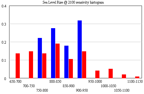
The sample would have to be bigger to reveal the true distribution (particularly for the “overconfident” version in blue), but the qualitative result is unlikely to change. All runs lie above the IPCC range (.26-.59), which excludes ice dynamics.
Continue reading “Sea Level Rise – VI – The Bottom Line (Almost)”
To take a look at the payoff surface, we need to do more than the naive calibrations I’ve used so far. Those were adequate for choosing constant terms that aligned the model trajectory with the data, given a priori values of a and tau. But that approach could give flawed estimates and confidence bounds when used to estimate the full system.
Elaborating on my comment on estimation at the end of Part II, consider a simplified description of our model, in discrete time:
(1) sea_level(t) = f(sea_level(t-1), temperature, parameters) + driving_noise(t)
(2) measured_sea_level(t) = sea_level(t) + measurement_noise(t)
The driving noise reflects disturbances to the system state: in this case, random perturbations to sea level. Measurement noise is simply errors in assessing the true state of global sea level, which could arise from insufficient coverage or accuracy of instruments. In the simple case, where driving and measurement noise are both zero, measured and actual sea level are the same, so we have the following system:
(3) sea_level(t) = f(sea_level(t-1), temperature, parameters)
In this case, which is essentially what we’ve assumed so far, we can simply initialize the model, feed it temperature, and simulate forward in time. We can estimate the parameters by adjusting them to get a good fit. However, if there’s driving noise, as in (1), we could be making a big mistake, because the noise may move the real-world state of sea level far from the model trajectory, in which case we’d be using the wrong value of sea_level(t-1) on the right hand side of (1). In effect, the model would blunder ahead, ignoring most of the data.
In this situation, it’s better to use ordinary least squares (OLS), which we can implement by replacing modeled sea level in (1) with measured sea level:
(4) sea_level(t) = f(measured_sea_level(t-1), temperature, parameters)
In (4), we’re ignoring the model rather than the data. But that could be a bad move too, because if measurement noise is nonzero, the sea level data could be quite different from true sea level at any point in time.
The point of the Kalman Filter is to combine the model and data estimates of the true state of the system. To do that, we simulate the model forward in time. Each time we encounter a data point, we update the model state, taking account of the relative magnitude of the noise streams. If we think that measurement error is small and driving noise is large, the best bet is to move the model dramatically towards the data. On the other hand, if measurements are very noisy and driving noise is small, better to stick with the model trajectory, and move only a little bit towards the data. You can test this in the model by varying the driving noise and measurement error parameters in SyntheSim, and watching how the model trajectory varies.
The discussion above is adapted from David Peterson’s thesis, which has a more complete mathematical treatment. The approach is laid out in Fred Schweppe’s book, Uncertain Dynamic Systems, which is unfortunately out of print and pricey. As a substitute, I like Stengel’s Optimal Control and Estimation.
An example of Kalman Filtering in everyday devices is GPS. A GPS unit is designed to estimate the state of a system (its location in space) using noisy measurements (satellite signals). As I understand it, GPS units maintain a simple model of the dynamics of motion: my expected position in the future equals my current perceived position, plus perceived velocity times time elapsed. It then corrects its predictions as measurements allow. With a good view of four satellites, it can move quickly toward the data. In a heavily-treed valley, it’s better to update the predicted state slowly, rather than giving jumpy predictions. I don’t know whether handheld GPS units implement it, but it’s possible to estimate the noise variances from the data and model, and adapt the filter corrections on the fly as conditions change.
So far, I’ve established that the qualitative results of Rahmstorf (R) and Grinsted (G) can be reproduced. Exact replication has been elusive, but the list of loose ends (unresolved differences in data and so forth) is long enough that I’m not concerned that R and G made fatal errors. However, I haven’t made much progress against the other items on my original list of questions:
At this point I’ll reveal my working hypotheses (untested so far):
Starting from the Rahmstorf (R) parameterization (tested, but not exhaustively), let’s turn to Grinsted et al (G).
First, I’ve made a few changes to the model and supporting spreadsheet. The previous version ran with a small time step, because some of the tide data was monthly (or less). That wasted clock cycles and complicated computation of residual autocorrelations and the like. In this version, I binned the data into an annual window and shifted the time axes so that the model will use the appropriate end-of-year points (when Vensim has data with a finer time step than the model, it grabs the data point nearest each time step for comparison with model variables). I also retuned the mean adjustments to the sea level series. I didn’t change the temperature series, but made it easier to use pure-Moberg (as G did). Those changes necessitate a slight change to the R calibration, so I changed the default parameters to reflect that.
Now it should be possible to plug in G parameters, from Table 1 in the paper. First, using Moberg: a = 1290 (note that G uses meters while I’m using mm), tau = 208, b = 770 (corresponding with T0=-0.59), initial sea level = -2. The final time for the simulation is set to 1979, and only Moberg temperature data are used. The setup for this is in change files, GrinstedMoberg.cin and MobergOnly.cin.
Picking up where I left off, with model and data assembled, the next step is to calibrate, to see whether the Rahmstorf (R) and Grinsted (G) results can be replicated. I’ll do that the easy way, and the right way.
An easy first step is to try the R approach, assuming that the time constant tau is long and that the rate of sea level rise is proportional to temperature (or the delta against some preindustrial equilibrium).
Rahmstorf estimated the temperature-sea level rise relationship by regressing a smoothed rate of sea level rise against temperature, and found a slope of 3.4 mm/yr/C.
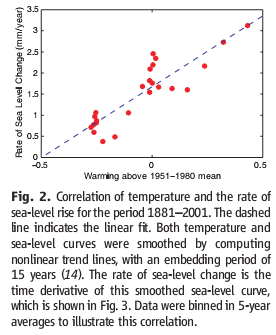
A recent post by Stefan Rahmstorf at RealClimate discusses a new paper on sea level projections by Grinsted, Moore and Jevrejeva. This paper comes at an interesting time, because we’ve just been discussing sea level projections in the context of our ongoing science review of the C-ROADS model. In C-ROADS, we used Rahmstorf’s earlier semi-empirical model, which yields higher sea level rise than AR4 WG1 (the latter leaves out ice sheet dynamics). To get a better handle on the two papers, I compared a replication of the Rahmstorf model (from John Sterman, implemented in C-ROADS) with an extension to capture Grinsted et al. This post (in a few parts) serves as both an assessment of the models and a bit of a tutorial on data analysis with Vensim.
My primary goal here is to develop an opinion on four questions:
I’ve been watching a variety of explanations of the financial crisis. As a wise friend noticed, the only thing in short supply is acceptance of responsibility. I’ve seen theories that place the seminal event as far back as the Carter administration. Does that make sense, causally?
In a formal sense, it might in some cases. I could have inhaled a carcinogen a decade ago that only leads to cancer a decade from now, without any outside triggers. But I think that sort of system is a rarity. As a practical matter, we have to look elsewhere.
Socioeconomic systems are at a constant slow boil, with many potential threats existing below the threshold of imminent danger at any given time. Occasionally, one grows exponentially and emerges as a real catastrophe. It seems like a surprise, because of the hockey stick behavior of growth (the French riddle of the lily pond again). However, most apparent low-level threats never emerge from the noise. They don’t have enough gain to grow fast, or they get shut down by some unsuspected negative feedback.