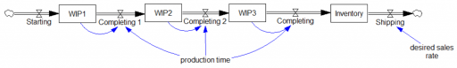
I’ve been approached several times recently with questions about stocks behaving badly. All involved a construction something like the following:
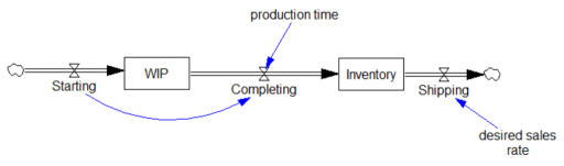
This is a simple inventory control system, in which I’ve short-circuited the production start feedback by making Starting exogenous and equal to the desired sales rate. Therefore, there are really only two interesting equations:
Shipping=desired sales rate
Units: widgets/Month

Completing=DELAY3( Starting, production time )
Units: widgets/Month
Notice that there’s a violation of standard practice here, in that there’s a flow-to-flow connection from Starting to Completing. This is due to the DELAY3 function, which is shorthand for an explicit 3rd-order delay:
The 3rd-order delay is often a realistic compromise between a 1st-order system, in which the first completions arrive too quickly after Starting, and a pipeline delay or conveyor, which has too little dispersion to represent an aggregation of many items. (See the Delay Sandbox and Erlang models for examples.)
So, how can we break this model?
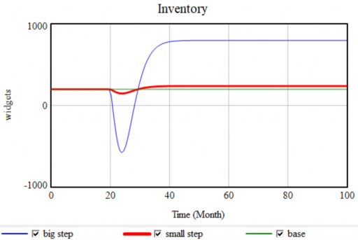
I always like to start with some tests in Synthesim. A good one is to stress the system with a step in the desired sales rate, here from 100 to 120. You can immediately spot a problem:
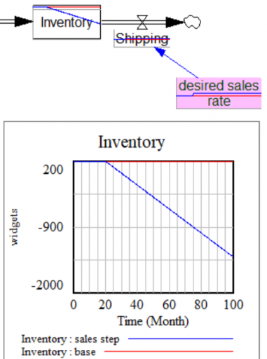
Inventory goes negative, because Shipping proceeds, even when inventory is exhausted. That can’t happen in reality, but it happens here because Shipping is not a function of Inventory. There’s a simple fix:
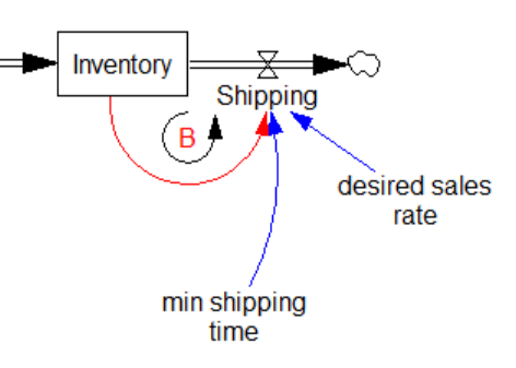
Shipping=MIN(desired sales rate, Inventory/min shipping time)
Units: widgets/Month
Above, min shipping time is a time constant representing the minimum time needed to deplete inventory. It’s common to set min shipping time = TIME STEP in situations where you want to prevent negative inventory, and the precise dynamics of inventory exhaustion are not central to the model. (If it matters, see Dynamics of the Last Twinkie.)
This is FONFOO. The “first order negative feedback” refers to the balancing loop created by the Inventory/min shipping time term in the fixed equation:
The tricky thing about this situation is that if Starting had been endogenous, the negative inventory problem would have been much harder to spot. Here’s the same model with a simple decision rule for Starting that maintains Inventory and WIP and desired levels:
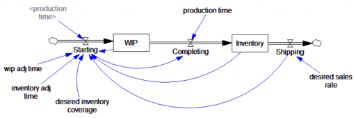
Now, a modest step in sales doesn’t cause negative inventory, as long as the production process can replenish it in time. It takes a huge step (from 100 to 400 widgets/month) to reveal the problem:
This means that experiments on a model as a whole may not reveal problems that lurk in the details of the model, unless they’re quite extreme. I recommend extreme tests, but prevention is more important. Simply make it a habit to implement FONFOO everywhere, and you won’t have problems. (Note that we could automate this in Vensim, but we don’t, because doing so can easily mask other formulation problems, fall short of the control that’s really needed, or impede situations in which nonphysical stocks are intentionally negative.)
Now let’s take a look at the 3rd-order production delay surrounding WIP. As presented above, it works fine – it’s mathematically equivalent to the explicit 3rd-order aging chain. However, there are consistency issues to be aware of. Consider the following augmentation of the structure, representing stock losses (the flow of Breaking) from WIP:
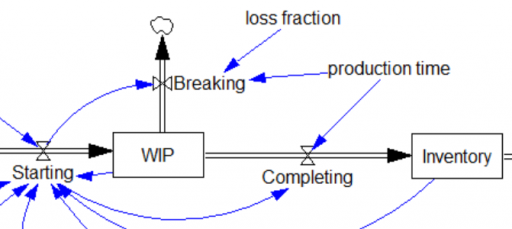
Completing=DELAY3( Starting, production time )
Units: widgets/Month
Breaking=DELAY3(Starting*loss fraction,production time)
Units: widgets/Month
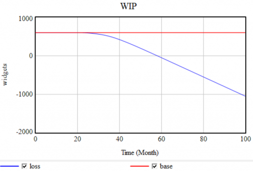
Completing is still a delayed function of Starting. But Completing is not directly aware of WIP and therefore unaware of the consequences of Breaking. This is a violation of FONFOO because the DELAY3 function contains internal states that are independent of the WIP stock. Consider what happens if the loss fraction is nonzero. In equilibrium, the output of DELAY3 is equal to the inflow. So, the outflow from WIP would be Breaking+Completing, which equals Starting+Starting*loss fraction, which is of course greater than starting for any nonzero loss.
A step in the loss function from 0 to 0.2 causes WIP to go negative:
Again, the remedy is simple. In most cases, you can keep the DELAY function if you ensure that the inflows and outflows are conserved. For example, adding a term:
Completing=DELAY3( Starting*(1-loss fraction), production time )
 Units: widgets/Month
 Breaking=DELAY3(Starting*loss fraction,production time)
 Units: widgets/Month
In some situations, it may be desirable to switch to an explicit aging chain in order to handle an idiosyncratic distribution of losses across the WIP process, or other complexities. Often arrays are useful for such purposes.
You may encounter the DELAY1 function in similar circumstances. DELAY1 is just like DELAY3, except that it’s first order. So, the system:
inflow = 10 ~ widgets/month
stock = INTEG(inflow-outflow, inflow*tau) ~ widgets
outflow = stock/tau ~ widgets/month
tau = 6 ~ months
is identical to the system:
inflow = 10 ~ widgets/month
stock = INTEG(inflow-outflow, inflow*tau) ~ widgets
outflow = DELAY1(inflow,tau) ~ widgets/month
tau = 6 ~ months
In this case, there’s really no reason to use the DELAY1 – it just obfuscates the first-order stock dynamics. However, there’s still a potential pitfall, which also applies to DELAY3. The initialization is important. The DELAY functions generally initialize their internal stocks in equilibrium, as if the inflow had been at its initial level historically. Therefore the stock above needs to be initialized the same way, to inflow*tau. If you want to use some other value, like zero, you need to use DELAY3i (or its equivalent) to set the stock and delay function to a consistent set of assumptions.
In reviewing other models, you may also find hybrid approaches, like:
inflow = 10 ~ widgets/month
stock = INTEG(inflow-outflow, inflow*tau) ~ widgets
outflow = DELAY1(stock/tau,tau) ~ widgets/month
tau = 6 ~ months
This is another FONFOO violation. The outflow is indeed a function of the stock, which ensures that the outflow eventually goes to zero when the stock is exhausted. But this does not create a 1st-order negative feedback loop; the DELAY1 contains an additional stock. So, this is SONFOO (second order negative feedback on the outflow), which might be useful for creating an oscillator, but won’t solve your supply chain problems.
If you make FONFOO a habit, you’ll have one less thing to worry about when you start exploring the interesting, complex behaviors of your models.