Model Library – Page 2

Misadventures with Little’s Law

I’ve been working on a vehicle fleet model, re-implementing a spreadsheet in Ventity, using dynamic cohorts.

The vehicle lifetime in the spreadsheet is 11 years, and it’s discrete. This means that every vehicle retires precisely 11 years after it’s put into service. This raised a red flag for me, because it represents a rather short vehicle lifetime. I know from work in other jurisdictions that the average life of a vehicle is more like 16-18 years typically (and getting longer as quality improves).

So, where does the 11 year figure come from? We’re not sure. Other published data for the region indicates an average vehicle age of 8.5 years, so it’s not that. A Ventana colleague pointed out that it might be a steady-state estimate from combining vehicle fleet data with new vehicle sales data:

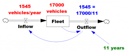
Given the data (red), assume that the vehicle stock is in equilibrium (inflow=outflow). Then it follows from Little’s Law that the average lifetime of vehicles must be 11 years. Little’s Law works regardless of the delay distribution, i.e. regardless of the delay order, but if you were formulating the fleet as a first-order system, that’s precisely how you’d write the outflow equation: outflow = fleet/lifetime, with lifetime=11 years.

… the long-term average number L of customers in a stationary system is equal to the long-term average effective arrival rate λ multiplied by the average time W that a customer spends in the system. – Wikipedia

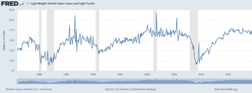
However, there’s a danger here. The system might not be in equilibrium. Then both the assumption of inflow=0utflow and the stationarity required in Little’s Law. Vehicle sales are, unfortunately, rather volatile, particularly around events like the 2008 recession:

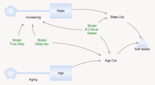
It’s tempting to use the average age of vehicles as another data point, but that turns out to be a bad idea. The average age of vehicles is sensitive to both variations in the inflow and the assumed distribution of the discard process. The following Ventity model illustrates this problem, using some of the same machinery as last week’s Erlang model.

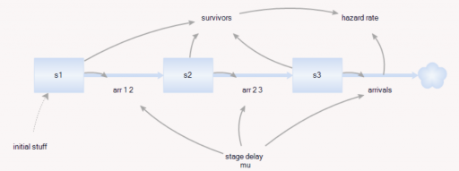
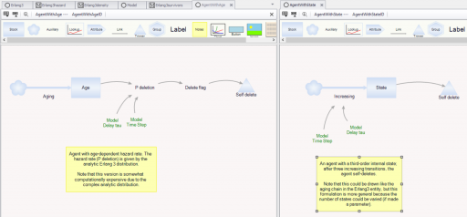
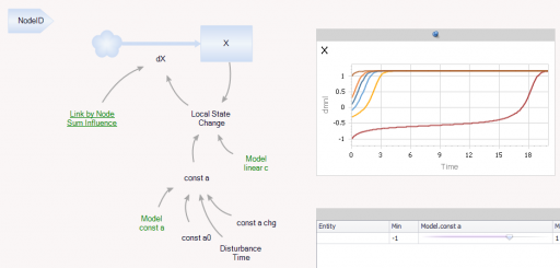
As before, there’s a population of entities (agents). Each has a cascade of N internal states, represented by a stock counter, and an age that increases continuously. An entity deletes itself when it’s too old, or its state count is too high.

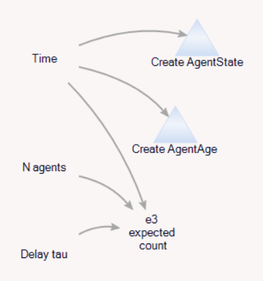
For accounting purposes, when an entity “dies” it records the event by incrementing counter stocks in the Model entity:

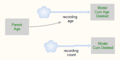
In this way, we can keep track of how old the average entity was at the time it deleted itself. This should be the average residence time in Little’s Law. We can also track the average age of existing entities, to see whether it’s the same.

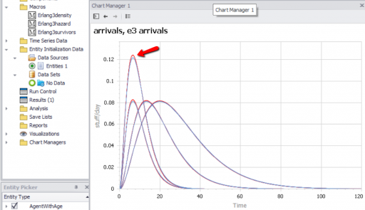
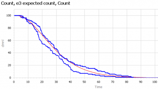
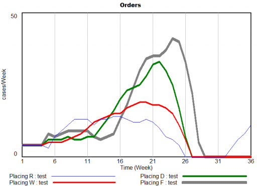
First, consider a very simple, very nonstationary special case, in which there’s no flow of entity turnover. There’s only an initial population of entities of age 0, who gradually leave the system. Here are three variants of that experiment:

Set Model.Delay tau = 50 and Model.Flow Start Time = 1000 to replicate this experiment.

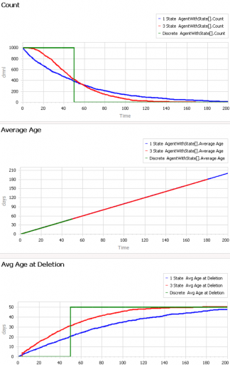
The blue line is the stochastic population analog of the classic first-order delay. The probability of a given entity departing is constant over time, as for radioactive decay. Therefore we get exponential decay, with count = N0*exp(-time/Delay tau). The red line is the third-order equivalent, yielding an Erlang 3 distribution. The green line is the pipeline delay equivalent, in which all entities self-delete at a specified age, rather than with a random distribution. Therefore the population steps from 1000 to 0 at time 50.

The two lower panels compare the average age of surviving entities (middle) to the average age at which entities self-delete (bottom). At bottom, you can see that all variants eventually converge to (roughly) the expected 50-year entity lifespan. However, each trajectory initially indicates a shorter lifespan. This is due to a form of censoring bias – at a given point in time, the longest-lived entities have not yet been observed.

The middle panel indicates how average age can mislead. In this case, age=time for all entities, and therefore the average age increases linearly, even though the expected residence time is constant.

At the opposite extreme, here’s an experiment with a constant flow of new agents, so that the system is in equilibrium after a few time constants:

Set Model.Delay tau = 20 and Model.Flow Start Time = 0 to replicate this experiment.

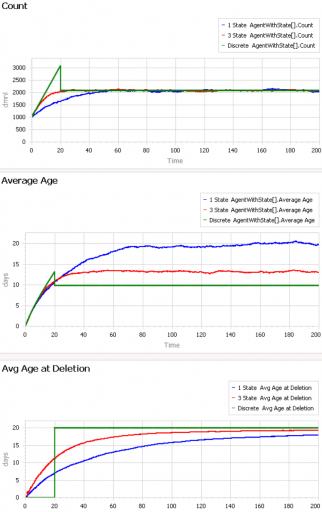
After the initial transient has died out (by time 20 to 60), all 3 residence times (age at deletion) converge to the expected value of 20. But notice the ages. They converge, too, but the value is dependent on the distribution. For the 1st-order system (blue), the average age does equal the average residence time of 20 years. But the pipeline system (green) has an average age that’s half that, at 10 years. This makes sense, if you think about an equilibrium population composed of a uniform mix of ages between 0 and 20 years. The 3rd-order system is in between.

This uncertain relationship between age and residence time means that we can’t use the average age of the vehicle fleet to determine the rate of vehicle turnover. That’s too bad, because age is the one statistic that’s easy to compute from a database of vehicle registrations. To know more, we have to start making inferences about the inflows and outflows – but that’s tricky if data coverage varies with time. Unfortunately, this is a number that we care about, because the residence time of vehicles in the system is an important driver of future penetration of low-carbon technologies.

The model: AgentAge2.zip

The Delay Sandbox can be used to explore similar phenomena in a continuous, aggregate, deterministic setting.

Aging Chains and the Erlang Distribution

My Delay Sandbox model illustrates the correspondence between Nth-order delays and the Erlang distribution (among other things).

Delay Sandbox

This model provides some similar insights – this time in Ventity. It’s a hybrid of classic continuous SD and agent equivalents.

First, the Erlang3 entitytype compares the classic 3rd-order aging chain’s behavior to analytical equivalents, as in the Delay Sandbox. The analytic values are computed in a set of Ventity’s new macros:

Notice that the variances, which arise from Euler integration with a finite time step, are small enough to be uninteresting.

Second, the model compares the dynamics of discrete agent populations to the analytic Erlang results. To do this, the Model entity creates populations of agents at time 0, and (for comparison) computes the expected surviving population according to the Erlang distribution:

The agents live for a time, then self-delete according to two different strategies:

On the left, an agent tracks its own age, and has an age-specific probability of mortality (again, thanks to the hazard rate of the Erlang distribution). On the right, an agent has a state counter, and mortality occurs when the number of state transitions reaches 3.

We can then compare the surviving agent populations (blue) to the Erlang expectation (red):

When the population is small (above, 100), there’s some stochastic variation around the expected result. But for larger populations, the difference is negligible.

The model: Erlang3 4 (2).zip

Coupled Catastrophes

I ran across this cool article on network dynamics, and thought the model would be an interesting application for Ventity:

Coupled catastrophes: sudden shifts cascade and hop among interdependent systems

Charles D. Brummitt, George Barnett and Raissa M. D’Souza

Abstract

An important challenge in several disciplines is to understand how sudden changes can propagate among coupled systems. Examples include the synchronization of business cycles, population collapse in patchy ecosystems, markets shifting to a new technology platform, collapses in prices and in confidence in financial markets, and protests erupting in multiple countries. A number of mathematical models of these phenomena have multiple equilibria separated by saddle-node bifurcations. We study this behaviour in its normal form as fast–slow ordinary differential equations. In our model, a system consists of multiple subsystems, such as countries in the global economy or patches of an ecosystem. Each subsystem is described by a scalar quantity, such as economic output or population, that undergoes sudden changes via saddle-node bifurcations. The subsystems are coupled via their scalar quantity (e.g. trade couples economic output; diffusion couples populations); that coupling moves the locations of their bifurcations. The model demonstrates two ways in which sudden changes can propagate: they can cascade (one causing the next), or they can hop over subsystems. The latter is absent from classic models of cascades. For an application, we study the Arab Spring protests. After connecting the model to sociological theories that have bistability, we use socioeconomic data to estimate relative proximities to tipping points and Facebook data to estimate couplings among countries. We find that although protests tend to spread locally, they also seem to ‘hop’ over countries, like in the stylized model; this result highlights a new class of temporal motifs in longitudinal network datasets.

Ventity makes sense here because the system consists of a network of coupled states. Ventity makes it easy to represent a wide variety of network architectures. This means there are two types of entities in the system: “Nodes” and “Couplings.”

The Node entitytype contains a single state (X), with local feedback, as well as a remote influence from Coupling and a few global parameters referenced from the Model entity:

Continue reading “Coupled Catastrophes”

Opiod Epidemic Dynamics

I ran across an interesting dynamic model of the opioid epidemic that makes a good target for replication and critique:

Prevention of Prescription Opioid Misuse and Projected Overdose Deaths in the United States

Qiushi Chen; Marc R. Larochelle; Davis T. Weaver; et al.

Importance  Deaths due to opioid overdose have tripled in the last decade. Efforts to curb this trend have focused on restricting the prescription opioid supply; however, the near-term effects of such efforts are unknown.

Objective  To project effects of interventions to lower prescription opioid misuse on opioid overdose deaths from 2016 to 2025.

Design, Setting, and Participants  This system dynamics (mathematical) model of the US opioid epidemic projected outcomes of simulated individuals who engage in nonmedical prescription or illicit opioid use from 2016 to 2025. The analysis was performed in 2018 by retrospectively calibrating the model from 2002 to 2015 data from the National Survey on Drug Use and Health and the Centers for Disease Control and Prevention.

…

Conclusions and Relevance  This study’s findings suggest that interventions targeting prescription opioid misuse such as prescription monitoring programs may have a modest effect, at best, on the number of opioid overdose deaths in the near future. Additional policy interventions are urgently needed to change the course of the epidemic.

The model is fully described in supplementary content, but unfortunately it’s implemented in R and described in Greek letters, so it can’t be run directly:

That’s actually OK with me, because I think I learn more from implementing the equations myself than I do if someone hands me a working model.

While R gives you access to tremendous tools, I think it’s not a good environment for designing and testing dynamic models of significant size. You can’t easily inspect everything that’s going on, and there’s no easy facility for interactive testing. So, I was curious whether that would prove problematic in this case, because the model is small.

Here’s what it looks like, replicated in Vensim:

It looks complicated, but it’s not complex. It’s basically a cascade of first-order delay processes: the outflow from each stock is simply a fraction per time. There are no large-scale feedback loops. Continue reading “Opiod Epidemic Dynamics”

Biological Dynamics of Stress Response

At ISDC 2018, we gave the Dana Meadows Award for best student paper to Gizem Aktas, for Modeling the Biological Mechanisms that Determine the Dynamics of Stress Response of the Human Body (with Yaman Barlas). This is a very interesting paper that elegantly synthesizes literature on stress, mood, and hormone interactions. I plan to write more about it later, but for the moment, here’s the model for your exploration.

The dynamic stress response of the human body to stressors is produced by nonlinear interactions among its physiological sub-systems. The evolutionary function of the response is to enable the body to cope with stress. However, depending on the intensity and frequency of the stressors, the mechanism may lose its function and the body can go into a pathological state. Three subsystems of the body play the most essential role in the stress response: endocrine, immune and neural systems. We constructed a simulation model of these three systems to imitate the stress response under different types of stress stimuli. Cortisol, glucocorticoid receptors, proinflammatory cytokines, serotonin, and serotonin receptors are the main variables of the model. Using both qualitative and quantitative physiological data, the model is structurally and behaviorally well-validated. In subsequent scenario runs, we have successfully replicated the development of major depression in the body. More interestingly, the model can present quantitative representation of some very well acknowledged qualitative hypotheses about the stress response of the body. This is a novel quantitative step towards the comprehension of stress response in relation with other disorders, and it provides us with a tool to design and test treatment methods.

The original is a STELLA model; here I’ve translated it to Vensim and made some convenience upgrades. I used the forthcoming XMILE translation in Vensim to open the model. You get an ugly diagram (due to platform differences and XMILE’s lack of support for flow-clouds), but it’s functional enough to browse. I cleaned up the diagrams and moved them into multiple views to take better advantage of Vensim’s visual approach.

Continue reading “Biological Dynamics of Stress Response”

Dynamic Cohorts

This is the model library entry for my ISDC 2017 plenary paper with Larry Yeager on dynamic cohorts in Ventity:

Dynamic cohorts: a new approach to managing detail

While it is desirable to minimize the complexity of a model, some problems require the detailed representation of heterogeneous subgroups, where nonlinearities prevent aggregation or explicit chronological aging is needed. It is desirable to have a representation that avoids burdening the modeler or user computationally or cognitively. Eberlein & Thompson (2013) propose continuous cohorting, a novel solution to the cohort blending problem in population modeling, and test it against existing aging chain and cohort-shifting approaches. Continuous cohorting prevents blending of ages and other properties, at at some cost in complexity.

We propose another new solution, dynamic cohorts, that prevents blending with a comparatively low computational burden. More importantly, the approach simplifies the representation of distinct age, period and cohort effects and representation of dynamics other than the aging process, like migration and attribute coflows. By encapsulating the lifecycle of a representative cohort in a single entity, rather than dispersing it across many states over time, it makes it easier to develop and explain the model structure.

Paper: Dynamic Cohorts P1363.pdf

Models: Dynamic Cohorts S1363.zip

Presentation slides: Dynamic Cohorts Fid Ventana v2b.pdf

I’ve previously written about this here.

The Beer Game

The Beer Game is the classic business game in system dynamics, demonstrating just how tricky it can be to manage a seemingly-simple system with delays and feedback. It’s a great icebreaker for teams, because it makes it immediately clear that catastrophes happen endogenously and fingerpointing is useless.

The system demonstrates amplification, aka the bullwhip effect, in supply chains. John Sterman analyzes the physical and behavioral origins of underperformance in the game in this Management Science paper. Steve Graves has some nice technical observations about similar systems in this MSOM paper.

Here are two versions that are close to the actual board game and the Sterman article:

Beer Game Fiddaman NoSubscripts.zip

This version doesn’t use arrays, and therefore should be usable in Vensim PLE. It includes a bunch of .cin files that implement the (calibrated) decision heuristics of real teams of the past, as well as some sensitivity and optimization control files.

Beer Game Fiddaman Array.zip

This version does use arrays to represent the levels of the supply chain. That makes it a little harder to grasp, but much easier to modify if you want to add or remove levels from the system or conduct optimization experiments. It requires Vensim Pro or DSS, or the Model Reader.

Polynomials & Interpolating Functions for Decision Rules

Sometimes it’s useful to have a way to express a variable as a flexible function of time, so that you can find the trajectory that maximizes some quantity like profit or fit to data. A caveat: this is not generally the best thing to do. A simple feedback rule will be more robust to rescaling and uncertainty and more informative than a function of time. However, there are times when it’s useful for testing or data approximation to have an open-loop decision rule. The attached models illustrate some options.

If you have access to arrays in Vensim, the simplest is to use the VECTOR LOOKUP function, which reads a subscripted table of values with interpolation. However, that has two limitations: a uniform time axis, and linear interpolation.

If you want a smooth function, a natural option is to pick a polynomial, like

y = a + b*t + c*t^2 + d*t^3 …

However, it can be a little fiddly to interpret the coefficients or get them to produce a desired behavior. The Legendre polynomials provide a basis with nicer scaling, which still recovers the basic linear, quadratic, cubic (etc.) terms when needed. (In terms of my last post, their improved properties make them less sloppy.)

You can generalize these to 2 dimensions by taking tensor products of the 1D series. Another option is to pick the first n terms of Pascal’s triangle. These yield essentially the same result, and either way, things get complex fast.

Back to 1D series, what if you want to express the values as a sequence of x-y points, with smooth interpolation, rather than arcane coefficients? One option is the Lagrange interpolating polynomial. It’s simple to implement, and has continuous derivatives, but it’s an N^2 problem and therefore potentially compute-intensive. It might also behave badly outside its interval, or inside due to ringing.

Probably the best choice for a smooth trajectory specified by x-y points (and optionally, the slope at each point) is a cubic spline or Bezier curve.

Polynomials1.mdl – simple smooth functions, Legendre, Lagrange and spline, runs in any version of Vensim

InterpolatingArrays.mdl InterpolatingArrays.vpm – array functions, VECTOR LOOKUP, Lagrange and spline, requires Pro/DSS or the free Reader

Thyroid Dynamics

Quite a while back, I posted about the dynamics of the thyroid and its interactions with other systems.

That was a conceptual model; this is a mathematical model. This is a Vensim replication of:

Marisa Eisenberg, Mary Samuels, and Joseph J. DiStefano III

Extensions, Validation, and Clinical Applications of a Feedback Control System Simulator of the Hypothalamo-Pituitary-Thyroid Axis

Background:We upgraded our recent feedback control system (FBCS) simulation model of human thyroid hormone (TH) regulation to include explicit representation of hypothalamic and pituitary dynamics, and up-dated TH distribution and elimination (D&E) parameters. This new model greatly expands the range of clinical and basic science scenarios explorable by computer simulation.

Methods: We quantified the model from pharmacokinetic (PK) and physiological human data and validated it comparatively against several independent clinical data sets. We then explored three contemporary clinical issues with the new model: …

… These results highlight how highly nonlinear feedback in the hypothalamic-pituitary-thyroid axis acts to maintain normal hormone levels, even with severely reduced TSH secretion.

THYROID
Volume 18, Number 10, 2008
DOI: 10.1089=thy.2007.0388

This version is a superset of the authors’ earlier 2006 model, and closely reproduces that with a few parameter changes.

L-T4 Bioequivalence and Hormone Replacement Studies via Feedback Control Simulations

THYROID
Volume 16, Number 12, 2006

The model is used in:

TSH-Based Protocol, Tablet Instability, and Absorption Effects on L-T4 Bioequivalence

THYROID
Volume 19, Number 2, 2009
DOI: 10.1089=thy.2008.0148

This works with any Vensim version:

thyroid 2008 d.mdl

thyroid 2008 d.vpm